DAR_analysis

workflowr

• Summary
• Checks
• Past versions

Last updated: 2025-07-22

Checks: 7 0

Knit directory: ATAC_learning/

This reproducible R Markdown analysis was created with workflowr (version 1.7.1). The Checks tab describes the reproducibility checks that were applied when the results were created. The Past versions tab lists the development history.

---

R Markdown file: up-to-date

Great! Since the R Markdown file has been committed to the Git repository, you know the exact version of the code that produced these results.

Environment: empty

Great job! The global environment was empty. Objects defined in the global environment can affect the analysis in your R Markdown file in unknown ways. For reproduciblity it’s best to always run the code in an empty environment.

Seed: set.seed(20231016)

The command set.seed(20231016) was run prior to running the code in the R Markdown file. Setting a seed ensures that any results that rely on randomness, e.g. subsampling or permutations, are reproducible.

Session information: recorded

Great job! Recording the operating system, R version, and package versions is critical for reproducibility.

Cache: none

Nice! There were no cached chunks for this analysis, so you can be confident that you successfully produced the results during this run.

File paths: relative

Great job! Using relative paths to the files within your workflowr project makes it easier to run your code on other machines.

Repository version: bbb553e

Great! You are using Git for version control. Tracking code development and connecting the code version to the results is critical for reproducibility.

The results in this page were generated with repository version bbb553e. See the Past versions tab to see a history of the changes made to the R Markdown and HTML files.

Note that you need to be careful to ensure that all relevant files for the analysis have been committed to Git prior to generating the results (you can use wflow_publish or wflow_git_commit). workflowr only checks the R Markdown file, but you know if there are other scripts or data files that it depends on. Below is the status of the Git repository when the results were generated:

Ignored files:
    Ignored:    .RData
    Ignored:    .Rhistory
    Ignored:    .Rproj.user/
    Ignored:    analysis/H3K27ac_integration_noM.Rmd
    Ignored:    data/ACresp_SNP_table.csv
    Ignored:    data/ARR_SNP_table.csv
    Ignored:    data/All_merged_peaks.tsv
    Ignored:    data/CAD_gwas_dataframe.RDS
    Ignored:    data/CTX_SNP_table.csv
    Ignored:    data/Collapsed_expressed_NG_peak_table.csv
    Ignored:    data/DEG_toplist_sep_n45.RDS
    Ignored:    data/FRiP_first_run.txt
    Ignored:    data/Final_four_data/
    Ignored:    data/Frip_1_reads.csv
    Ignored:    data/Frip_2_reads.csv
    Ignored:    data/Frip_3_reads.csv
    Ignored:    data/Frip_4_reads.csv
    Ignored:    data/Frip_5_reads.csv
    Ignored:    data/Frip_6_reads.csv
    Ignored:    data/GO_KEGG_analysis/
    Ignored:    data/HF_SNP_table.csv
    Ignored:    data/Ind1_75DA24h_dedup_peaks.csv
    Ignored:    data/Ind1_TSS_peaks.RDS
    Ignored:    data/Ind1_firstfragment_files.txt
    Ignored:    data/Ind1_fragment_files.txt
    Ignored:    data/Ind1_peaks_list.RDS
    Ignored:    data/Ind1_summary.txt
    Ignored:    data/Ind2_TSS_peaks.RDS
    Ignored:    data/Ind2_fragment_files.txt
    Ignored:    data/Ind2_peaks_list.RDS
    Ignored:    data/Ind2_summary.txt
    Ignored:    data/Ind3_TSS_peaks.RDS
    Ignored:    data/Ind3_fragment_files.txt
    Ignored:    data/Ind3_peaks_list.RDS
    Ignored:    data/Ind3_summary.txt
    Ignored:    data/Ind4_79B24h_dedup_peaks.csv
    Ignored:    data/Ind4_TSS_peaks.RDS
    Ignored:    data/Ind4_V24h_fraglength.txt
    Ignored:    data/Ind4_fragment_files.txt
    Ignored:    data/Ind4_fragment_filesN.txt
    Ignored:    data/Ind4_peaks_list.RDS
    Ignored:    data/Ind4_summary.txt
    Ignored:    data/Ind5_TSS_peaks.RDS
    Ignored:    data/Ind5_fragment_files.txt
    Ignored:    data/Ind5_fragment_filesN.txt
    Ignored:    data/Ind5_peaks_list.RDS
    Ignored:    data/Ind5_summary.txt
    Ignored:    data/Ind6_TSS_peaks.RDS
    Ignored:    data/Ind6_fragment_files.txt
    Ignored:    data/Ind6_peaks_list.RDS
    Ignored:    data/Ind6_summary.txt
    Ignored:    data/Knowles_4.RDS
    Ignored:    data/Knowles_5.RDS
    Ignored:    data/Knowles_6.RDS
    Ignored:    data/LiSiLTDNRe_TE_df.RDS
    Ignored:    data/MI_gwas.RDS
    Ignored:    data/SNP_GWAS_PEAK_MRC_id
    Ignored:    data/SNP_GWAS_PEAK_MRC_id.csv
    Ignored:    data/SNP_gene_cat_list.tsv
    Ignored:    data/SNP_supp_schneider.RDS
    Ignored:    data/TE_info/
    Ignored:    data/TFmapnames.RDS
    Ignored:    data/all_TSSE_scores.RDS
    Ignored:    data/all_four_filtered_counts.txt
    Ignored:    data/aln_run1_results.txt
    Ignored:    data/anno_ind1_DA24h.RDS
    Ignored:    data/anno_ind4_V24h.RDS
    Ignored:    data/annotated_gwas_SNPS.csv
    Ignored:    data/background_n45_he_peaks.RDS
    Ignored:    data/cardiac_muscle_FRIP.csv
    Ignored:    data/cardiomyocyte_FRIP.csv
    Ignored:    data/col_ng_peak.csv
    Ignored:    data/cormotif_full_4_run.RDS
    Ignored:    data/cormotif_full_4_run_he.RDS
    Ignored:    data/cormotif_full_6_run.RDS
    Ignored:    data/cormotif_full_6_run_he.RDS
    Ignored:    data/cormotif_probability_45_list.csv
    Ignored:    data/cormotif_probability_45_list_he.csv
    Ignored:    data/cormotif_probability_all_6_list.csv
    Ignored:    data/cormotif_probability_all_6_list_he.csv
    Ignored:    data/datasave.RDS
    Ignored:    data/embryo_heart_FRIP.csv
    Ignored:    data/enhancer_list_ENCFF126UHK.bed
    Ignored:    data/enhancerdata/
    Ignored:    data/filt_Peaks_efit2.RDS
    Ignored:    data/filt_Peaks_efit2_bl.RDS
    Ignored:    data/filt_Peaks_efit2_n45.RDS
    Ignored:    data/first_Peaksummarycounts.csv
    Ignored:    data/first_run_frag_counts.txt
    Ignored:    data/full_bedfiles/
    Ignored:    data/gene_ref.csv
    Ignored:    data/gwas_1_dataframe.RDS
    Ignored:    data/gwas_2_dataframe.RDS
    Ignored:    data/gwas_3_dataframe.RDS
    Ignored:    data/gwas_4_dataframe.RDS
    Ignored:    data/gwas_5_dataframe.RDS
    Ignored:    data/high_conf_peak_counts.csv
    Ignored:    data/high_conf_peak_counts.txt
    Ignored:    data/high_conf_peaks_bl_counts.txt
    Ignored:    data/high_conf_peaks_counts.txt
    Ignored:    data/hits_files/
    Ignored:    data/hyper_files/
    Ignored:    data/hypo_files/
    Ignored:    data/ind1_DA24hpeaks.RDS
    Ignored:    data/ind1_TSSE.RDS
    Ignored:    data/ind2_TSSE.RDS
    Ignored:    data/ind3_TSSE.RDS
    Ignored:    data/ind4_TSSE.RDS
    Ignored:    data/ind4_V24hpeaks.RDS
    Ignored:    data/ind5_TSSE.RDS
    Ignored:    data/ind6_TSSE.RDS
    Ignored:    data/initial_complete_stats_run1.txt
    Ignored:    data/left_ventricle_FRIP.csv
    Ignored:    data/median_24_lfc.RDS
    Ignored:    data/median_3_lfc.RDS
    Ignored:    data/mergedPeads.gff
    Ignored:    data/mergedPeaks.gff
    Ignored:    data/motif_list_full
    Ignored:    data/motif_list_n45
    Ignored:    data/motif_list_n45.RDS
    Ignored:    data/multiqc_fastqc_run1.txt
    Ignored:    data/multiqc_fastqc_run2.txt
    Ignored:    data/multiqc_genestat_run1.txt
    Ignored:    data/multiqc_genestat_run2.txt
    Ignored:    data/my_hc_filt_counts.RDS
    Ignored:    data/my_hc_filt_counts_n45.RDS
    Ignored:    data/n45_bedfiles/
    Ignored:    data/n45_files
    Ignored:    data/other_papers/
    Ignored:    data/peakAnnoList_1.RDS
    Ignored:    data/peakAnnoList_2.RDS
    Ignored:    data/peakAnnoList_24_full.RDS
    Ignored:    data/peakAnnoList_24_n45.RDS
    Ignored:    data/peakAnnoList_3.RDS
    Ignored:    data/peakAnnoList_3_full.RDS
    Ignored:    data/peakAnnoList_3_n45.RDS
    Ignored:    data/peakAnnoList_4.RDS
    Ignored:    data/peakAnnoList_5.RDS
    Ignored:    data/peakAnnoList_6.RDS
    Ignored:    data/peakAnnoList_Eight.RDS
    Ignored:    data/peakAnnoList_full_motif.RDS
    Ignored:    data/peakAnnoList_n45_motif.RDS
    Ignored:    data/siglist_full.RDS
    Ignored:    data/siglist_n45.RDS
    Ignored:    data/summarized_peaks_dataframe.txt
    Ignored:    data/summary_peakIDandReHeat.csv
    Ignored:    data/test.list.RDS
    Ignored:    data/testnames.txt
    Ignored:    data/toplist_6.RDS
    Ignored:    data/toplist_full.RDS
    Ignored:    data/toplist_full_DAR_6.RDS
    Ignored:    data/toplist_n45.RDS
    Ignored:    data/trimmed_seq_length.csv
    Ignored:    data/unclassified_full_set_peaks.RDS
    Ignored:    data/unclassified_n45_set_peaks.RDS
    Ignored:    data/xstreme/

Untracked files:
    Untracked:  RNA_seq_integration.Rmd
    Untracked:  Rplot.pdf
    Untracked:  Sig_meta
    Untracked:  analysis/.gitignore
    Untracked:  analysis/AF_HF_SNP_DAR.Rmd
    Untracked:  analysis/AF_HF_SNP_DAR_logFC.Rmd
    Untracked:  analysis/Cormotif_analysis_testing diff.Rmd
    Untracked:  analysis/Diagnosis-tmm.Rmd
    Untracked:  analysis/Expressed_RNA_associations.Rmd
    Untracked:  analysis/LFC_corr.Rmd
    Untracked:  analysis/SVA.Rmd
    Untracked:  analysis/Tan2020.Rmd
    Untracked:  analysis/making_master_peaks_list.Rmd
    Untracked:  analysis/my_hc_filt_counts.csv
    Untracked:  code/Concatenations_for_export.R
    Untracked:  code/IGV_snapshot_code.R
    Untracked:  code/LongDARlist.R
    Untracked:  code/just_for_Fun.R
    Untracked:  my_plot.pdf
    Untracked:  my_plot.png
    Untracked:  output/cormotif_probability_45_list.csv
    Untracked:  output/cormotif_probability_all_6_list.csv
    Untracked:  setup.RData

Unstaged changes:
    Modified:   ATAC_learning.Rproj
    Modified:   analysis/AC_shared_analysis.Rmd
    Modified:   analysis/AF_HF_SNPs.Rmd
    Modified:   analysis/Cardiotox_SNPs.Rmd
    Modified:   analysis/Cormotif_analysis.Rmd
    Modified:   analysis/DOX_DAR_heatmap.Rmd
    Modified:   analysis/H3K27ac_initial_QC.Rmd
    Modified:   analysis/H3K27ac_integration.Rmd
    Modified:   analysis/Jaspar_motif.Rmd
    Modified:   analysis/Jaspar_motif_DAR.Rmd
    Modified:   analysis/Jaspar_motif_ff.Rmd
    Modified:   analysis/TE_analysis_ALL_DAR.Rmd
    Modified:   analysis/TE_analysis_norm.Rmd
    Modified:   analysis/final_four_analysis.Rmd

Note that any generated files, e.g. HTML, png, CSS, etc., are not included in this status report because it is ok for generated content to have uncommitted changes.

---

These are the previous versions of the repository in which changes were made to the R Markdown (analysis/DEG_analysis.Rmd) and HTML (docs/DEG_analysis.html) files. If you’ve configured a remote Git repository (see ?wflow_git_remote), click on the hyperlinks in the table below to view the files as they were in that past version.

File	Version	Author	Date	Message
Rmd	bbb553e	reneeisnowhere	2025-07-22	updates to genomic regions plot
html	30dc0d7	reneeisnowhere	2025-07-21	Build site.
Rmd	787abdb	reneeisnowhere	2025-07-21	updates
Rmd	26eb8eb	reneeisnowhere	2025-06-23	adding updates
html	b377769	reneeisnowhere	2025-06-16	Build site.
Rmd	8843fef	reneeisnowhere	2025-06-16	fix plot names
html	7f3442d	reneeisnowhere	2025-06-13	Build site.
Rmd	352072c	reneeisnowhere	2025-06-13	updates to y and x axis
html	04d6841	reneeisnowhere	2025-06-12	Build site.
Rmd	601b63f	reneeisnowhere	2025-06-12	updates
html	eeaa3e6	reneeisnowhere	2025-06-09	Build site.
Rmd	7a30fff	reneeisnowhere	2025-06-09	updateing enrichment test
html	f0c5b69	reneeisnowhere	2025-06-05	Build site.
Rmd	23a3ce1	reneeisnowhere	2025-06-05	adding in DAR analysis
html	54e129a	reneeisnowhere	2025-05-15	Build site.
html	cf05574	reneeisnowhere	2025-05-14	Build site.
Rmd	19d6784	reneeisnowhere	2025-05-14	updates to volcano plots
html	4163890	reneeisnowhere	2025-05-12	Build site.
Rmd	9716d1a	reneeisnowhere	2025-05-12	updated with top3
html	cb0030e	reneeisnowhere	2025-05-08	Build site.
Rmd	df7eb88	reneeisnowhere	2025-05-08	spelling correction
html	5e6e462	reneeisnowhere	2025-05-07	Build site.
Rmd	d969893	reneeisnowhere	2025-05-07	updating new pages
html	fee3875	reneeisnowhere	2025-05-06	Build site.
Rmd	01178cf	reneeisnowhere	2025-05-06	adding in segment

---

library(tidyverse)
library(kableExtra)
library(broom)
library(RColorBrewer)
library(ChIPseeker)
library("TxDb.Hsapiens.UCSC.hg38.knownGene")
library("org.Hs.eg.db")
library(rtracklayer)
library(edgeR)
library(ggfortify)
library(limma)
library(readr)
library(BiocGenerics)
library(gridExtra)
library(VennDiagram)
library(scales)
library(BiocParallel)
library(ggpubr)
library(devtools)
library(eulerr)
library(ggsignif)
library(plyranges)
library(ggrepel)
library(ComplexHeatmap)
library(cowplot)
library(smplot2)
library(data.table)
library(ggVennDiagram)

Differential analysis

Loading counts matrix and making filtered matrix

raw_counts <- read_delim("data/Final_four_data/re_analysis/Raw_unfiltered_counts.tsv",delim="\t") %>% 
  column_to_rownames("Peakid") %>% 
  as.matrix()

lcpm <- cpm(raw_counts, log= TRUE)
  ### for determining the basic cutoffs
filt_raw_counts <- raw_counts[rowMeans(lcpm)> 0,]

filt_raw_counts_noY <- filt_raw_counts[!grepl("chrY",rownames(filt_raw_counts)),]
dim(filt_raw_counts_noY)

[1] 155557     48

Number of filtered regions without the y chromosome = 155557 regions

making the metadata form

annotation_mat <- data.frame(timeset=colnames(filt_raw_counts_noY)) %>%
  mutate(sample = timeset) %>% 
  separate(timeset, into = c("indv","trt","time"), sep= "_") %>% 
  mutate(time = factor(time, levels = c("3h", "24h"))) %>% 
  mutate(trt = factor(trt, levels = c("DOX","EPI", "DNR", "MTX", "TRZ", "VEH"))) %>% 
  mutate(indv=factor(indv, levels = c("A","B","C","D"))) %>% 
  mutate(trt_time=paste0(trt,"_",time))

prepare DGE object

group <- c( rep(c(1,2,3,4,5,6,7,8,9,10,11,12),4))
group <- factor(group, levels =c("1","2","3","4","5","6","7","8","9","10","11","12"))
dge <-  DGEList.data.frame(counts = filt_raw_counts_noY, group = group, genes = row.names(filt_raw_counts_noY))
dge <- calcNormFactors(dge)

dge$samples

          group lib.size norm.factors
D_DNR_24h     1 16022907    1.0239692
D_DNR_3h      2 12283494    0.9612342
D_DOX_24h     3 17860884    1.0367665
D_DOX_3h      4 13506791    1.0325656
D_EPI_24h     5 18628141    1.0327372
D_EPI_3h      6 11218019    1.0171289
D_MTX_24h     7 15070579    1.1107812
D_MTX_3h      8  8224116    1.0938773
D_TRZ_24h     9 13765197    0.9916489
D_TRZ_3h     10  9838944    1.0289011
D_VEH_24h    11 18137669    0.9855606
D_VEH_3h     12  5215243    1.1193711
A_DNR_24h     1 12446867    0.9913953
A_DNR_3h      2 13336679    0.9109168
A_DOX_24h     3 11024760    0.8994761
A_DOX_3h      4 11312301    0.9817107
A_EPI_24h     5 10054890    0.8306893
A_EPI_3h      6 13289458    0.8846067
A_MTX_24h     7 12051332    1.0488547
A_MTX_3h      8 19529308    0.9756453
A_TRZ_24h     9 11144980    0.8850322
A_TRZ_3h     10 10815793    0.9696953
A_VEH_24h    11 10644539    0.9044966
A_VEH_3h     12 10146179    1.0015305
B_DNR_24h     1  8695642    1.0170461
B_DNR_3h      2 11572135    0.8666718
B_DOX_24h     3  7780737    1.0039941
B_DOX_3h      4  6315637    0.8935147
B_EPI_24h     5  7912993    1.0275056
B_EPI_3h      6  7196001    0.9035920
B_MTX_24h     7  7434261    1.0947453
B_MTX_3h      8 10544429    0.8769442
B_TRZ_24h     9  6552039    0.9772581
B_TRZ_3h     10  6390372    0.9027404
B_VEH_24h    11  3521378    1.0063550
B_VEH_3h     12  4936492    1.0027569
C_DNR_24h     1 11796366    1.0773328
C_DNR_3h      2  6968392    1.0576684
C_DOX_24h     3  8352016    1.1219236
C_DOX_3h      4  5992702    1.0623451
C_EPI_24h     5  7970178    1.1143342
C_EPI_3h      6  5933236    1.0854547
C_MTX_24h     7  5584157    1.1803465
C_MTX_3h      8  9157251    1.0227009
C_TRZ_24h     9  5662913    1.0288892
C_TRZ_3h     10  4552166    1.0697477
C_VEH_24h    11  7597538    1.0237355
C_VEH_3h     12  6681133    1.0107246

Making model matrix

group_1 <- c(rep(c("DNR_24","DNR_3","DOX_24","DOX_3","EPI_24","EPI_3","MTX_24","MTX_3","TRZ_24","TRZ_3","VEH_24", "VEH_3"),4))

 mm <- model.matrix(~0 +group_1)
colnames(mm) <-  c("DNR_24", "DNR_3", "DOX_24","DOX_3","EPI_24", "EPI_3","MTX_24", "MTX_3", "TRZ_24","TRZ_3","VEH_24", "VEH_3")
mm

   DNR_24 DNR_3 DOX_24 DOX_3 EPI_24 EPI_3 MTX_24 MTX_3 TRZ_24 TRZ_3 VEH_24
1       1     0      0     0      0     0      0     0      0     0      0
2       0     1      0     0      0     0      0     0      0     0      0
3       0     0      1     0      0     0      0     0      0     0      0
4       0     0      0     1      0     0      0     0      0     0      0
5       0     0      0     0      1     0      0     0      0     0      0
6       0     0      0     0      0     1      0     0      0     0      0
7       0     0      0     0      0     0      1     0      0     0      0
8       0     0      0     0      0     0      0     1      0     0      0
9       0     0      0     0      0     0      0     0      1     0      0
10      0     0      0     0      0     0      0     0      0     1      0
11      0     0      0     0      0     0      0     0      0     0      1
12      0     0      0     0      0     0      0     0      0     0      0
13      1     0      0     0      0     0      0     0      0     0      0
14      0     1      0     0      0     0      0     0      0     0      0
15      0     0      1     0      0     0      0     0      0     0      0
16      0     0      0     1      0     0      0     0      0     0      0
17      0     0      0     0      1     0      0     0      0     0      0
18      0     0      0     0      0     1      0     0      0     0      0
19      0     0      0     0      0     0      1     0      0     0      0
20      0     0      0     0      0     0      0     1      0     0      0
21      0     0      0     0      0     0      0     0      1     0      0
22      0     0      0     0      0     0      0     0      0     1      0
23      0     0      0     0      0     0      0     0      0     0      1
24      0     0      0     0      0     0      0     0      0     0      0
25      1     0      0     0      0     0      0     0      0     0      0
26      0     1      0     0      0     0      0     0      0     0      0
27      0     0      1     0      0     0      0     0      0     0      0
28      0     0      0     1      0     0      0     0      0     0      0
29      0     0      0     0      1     0      0     0      0     0      0
30      0     0      0     0      0     1      0     0      0     0      0
31      0     0      0     0      0     0      1     0      0     0      0
32      0     0      0     0      0     0      0     1      0     0      0
33      0     0      0     0      0     0      0     0      1     0      0
34      0     0      0     0      0     0      0     0      0     1      0
35      0     0      0     0      0     0      0     0      0     0      1
36      0     0      0     0      0     0      0     0      0     0      0
37      1     0      0     0      0     0      0     0      0     0      0
38      0     1      0     0      0     0      0     0      0     0      0
39      0     0      1     0      0     0      0     0      0     0      0
40      0     0      0     1      0     0      0     0      0     0      0
41      0     0      0     0      1     0      0     0      0     0      0
42      0     0      0     0      0     1      0     0      0     0      0
43      0     0      0     0      0     0      1     0      0     0      0
44      0     0      0     0      0     0      0     1      0     0      0
45      0     0      0     0      0     0      0     0      1     0      0
46      0     0      0     0      0     0      0     0      0     1      0
47      0     0      0     0      0     0      0     0      0     0      1
48      0     0      0     0      0     0      0     0      0     0      0
   VEH_3
1      0
2      0
3      0
4      0
5      0
6      0
7      0
8      0
9      0
10     0
11     0
12     1
13     0
14     0
15     0
16     0
17     0
18     0
19     0
20     0
21     0
22     0
23     0
24     1
25     0
26     0
27     0
28     0
29     0
30     0
31     0
32     0
33     0
34     0
35     0
36     1
37     0
38     0
39     0
40     0
41     0
42     0
43     0
44     0
45     0
46     0
47     0
48     1
attr(,"assign")
 [1] 1 1 1 1 1 1 1 1 1 1 1 1
attr(,"contrasts")
attr(,"contrasts")$group_1
[1] "contr.treatment"

In this pipeline, I first run voom transformation, then estimate the intra-individual correlation. Next I do voom again with correlation info. I fit the linear model, define contrasts, then apply the contrasts and perform eBayes to get statistics.

y <- voom(dge, mm,plot =FALSE)

corfit <- duplicateCorrelation(y, mm, block = annotation_mat$indv)
 
v <- voom(dge, mm, block = annotation_mat$indv, correlation = corfit$consensus)

fit <- lmFit(v, mm, block = annotation_mat$indv, correlation = corfit$consensus)


cm <- makeContrasts(
  DNR_3.VEH_3 = DNR_3-VEH_3,
  DOX_3.VEH_3 = DOX_3-VEH_3,
  EPI_3.VEH_3 = EPI_3-VEH_3,
  MTX_3.VEH_3 = MTX_3-VEH_3,
  TRZ_3.VEH_3 = TRZ_3-VEH_3,
  DNR_24.VEH_24 =DNR_24-VEH_24,
  DOX_24.VEH_24= DOX_24-VEH_24,
  EPI_24.VEH_24= EPI_24-VEH_24,
  MTX_24.VEH_24= MTX_24-VEH_24,
  TRZ_24.VEH_24= TRZ_24-VEH_24,
  levels = mm)


fit2<- contrasts.fit(fit, contrasts=cm)

efit2 <- eBayes(fit2)

results = decideTests(efit2)

summary(results)

       DNR_3.VEH_3 DOX_3.VEH_3 EPI_3.VEH_3 MTX_3.VEH_3 TRZ_3.VEH_3
Down         10868        2244        7162         444           1
NotSig      132819      152084      141323      154753      155556
Up           11870        1229        7072         360           0
       DNR_24.VEH_24 DOX_24.VEH_24 EPI_24.VEH_24 MTX_24.VEH_24 TRZ_24.VEH_24
Down           39400         32313         32932         14182             0
NotSig         75562         90737         89056        131307        155557
Up             40595         32507         33569         10068             0

plotSA(efit2, main="Mean-Variance trend for final model")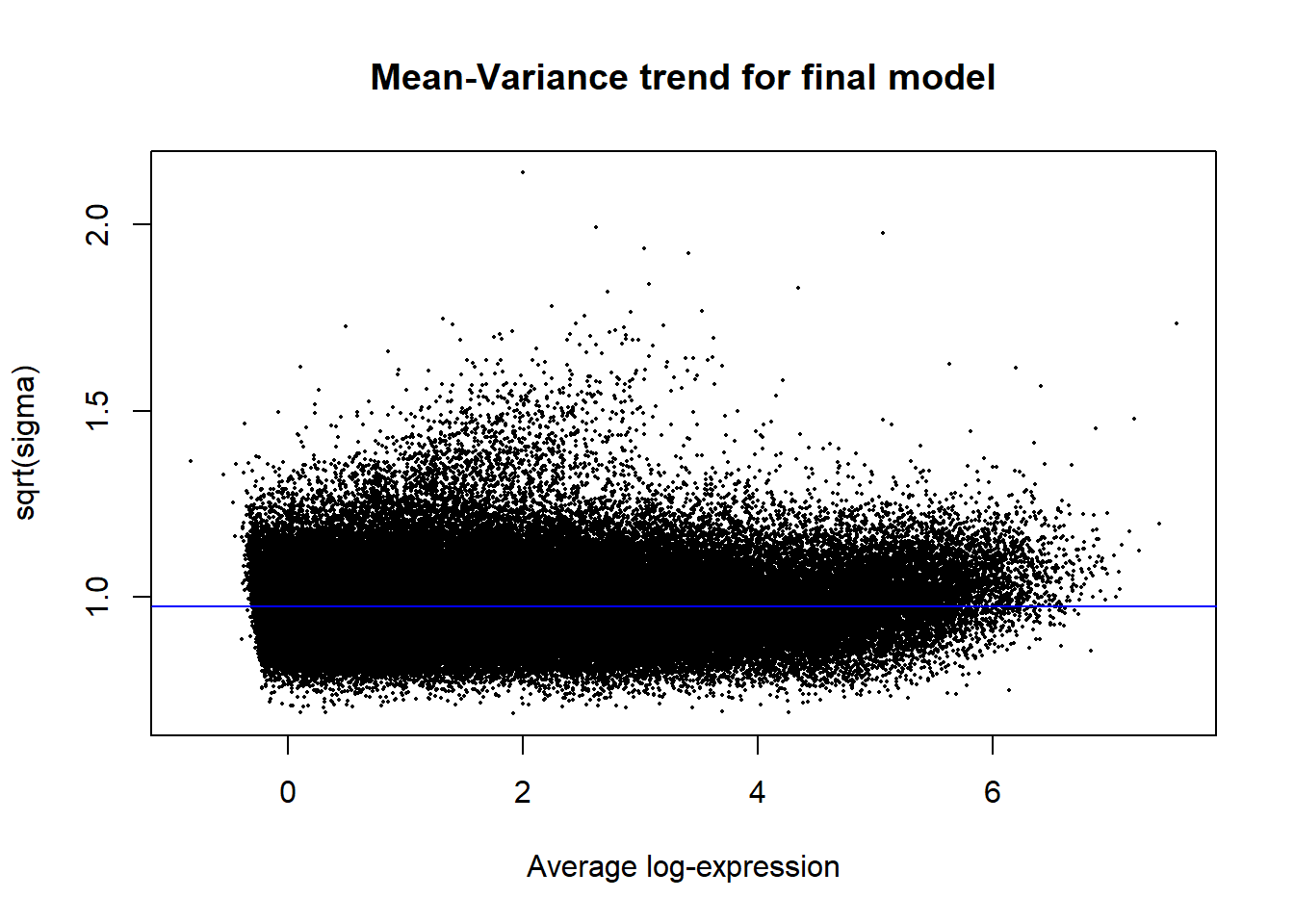

Past versions of unnamed-chunk-3-1.png

Version	Author	Date
fee3875	reneeisnowhere	2025-05-06

V.DNR_3.top= topTable(efit2, coef=1, adjust.method="BH", number=Inf, sort.by="p")
V.DOX_3.top= topTable(efit2, coef=2, adjust.method="BH", number=Inf, sort.by="p")
V.EPI_3.top= topTable(efit2, coef=3, adjust.method="BH", number=Inf, sort.by="p")
V.MTX_3.top= topTable(efit2, coef=4, adjust.method="BH", number=Inf, sort.by="p")
V.TRZ_3.top= topTable(efit2, coef=5, adjust.method="BH", number=Inf, sort.by="p")
V.DNR_24.top= topTable(efit2, coef=6, adjust.method="BH", number=Inf, sort.by="p")
V.DOX_24.top= topTable(efit2, coef=7, adjust.method="BH", number=Inf, sort.by="p")
V.EPI_24.top= topTable(efit2, coef=8, adjust.method="BH", number=Inf, sort.by="p")
V.MTX_24.top= topTable(efit2, coef=9, adjust.method="BH", number=Inf, sort.by="p")
V.TRZ_24.top= topTable(efit2, coef=10, adjust.method="BH", number=Inf, sort.by="p")


# plot_filenames <- c("V.DNR_3.top","V.DOX_3.top","V.EPI_3.top","V.MTX_3.top",
#                     "V.TRZ_.top","V.DNR_24.top","V.DOX_24.top","V.EPI_24.top",
#                     "V.MTX_24.top","V.TRZ_24.top")
# plot_files <- c( V.DNR_3.top,V.DOX_3.top,V.EPI_3.top,V.MTX_3.top,
#                     V.TRZ_3.top,V.DNR_24.top,V.DOX_24.top,V.EPI_24.top,
#                     V.MTX_24.top,V.TRZ_24.top)

save_list <- list("DNR_3"=V.DNR_3.top,"DOX_3"=V.DOX_3.top,"EPI_3"=V.EPI_3.top,"MTX_3"=V.MTX_3.top,"TRZ_3"=V.TRZ_3.top,"DNR_24"=V.DNR_24.top,"DOX_24"=V.DOX_24.top,"EPI_24"=V.EPI_24.top,"MTX_24"= V.MTX_24.top, "TRZ_24"=V.TRZ_24.top)

saveRDS(save_list,"data/Final_four_data/re_analysis/Toptable_results.RDS")

Volcano Plots

volcanosig <- function(df, psig.lvl) {
    df <- df %>% 
    mutate(threshold = ifelse(adj.P.Val > psig.lvl, "A", ifelse(adj.P.Val <= psig.lvl & logFC<=0,"B","C")))
      # ifelse(adj.P.Val <= psig.lvl & logFC >= 0,"B", "C")))
    ##This is where I could add labels, but I have taken out
    # df <- df %>% mutate(genelabels = "")
    # df$genelabels[1:topg] <- df$rownames[1:topg]
    
  ggplot(df, aes(x=logFC, y=-log10(P.Value))) + 
    ggrastr::geom_point_rast(aes(color=threshold))+
    # geom_text_repel(aes(label = genelabels), segment.curvature = -1e-20,force = 1,size=2.5,
    # arrow = arrow(length = unit(0.015, "npc")), max.overlaps = Inf) +
    #geom_hline(yintercept = -log10(psig.lvl))+
    xlab(expression("Log"[2]*" FC"))+
    ylab(expression("-log"[10]*"P Value"))+
    scale_color_manual(values = c("black", "red","blue"))+
    theme_cowplot()+
    ylim(0,25)+
    xlim(-6,6)+
    theme(legend.position = "none",
              plot.title = element_text(size = rel(1.5), hjust = 0.5),
              axis.title = element_text(size = rel(0.8))) 
}

v1 <- volcanosig(V.DNR_3.top, 0.05)+ ggtitle("DNR 3 hour")
v2 <- volcanosig(V.DNR_24.top, 0.05)+ ggtitle("DNR 24 hour")+ylab("")
v3 <- volcanosig(V.DOX_3.top, 0.05)+ ggtitle("DOX 3 hour")
v4 <- volcanosig(V.DOX_24.top, 0.05)+ ggtitle("DOX 24 hour")+ylab("")
v5 <- volcanosig(V.EPI_3.top, 0.05)+ ggtitle("EPI 3 hour")
v6 <- volcanosig(V.EPI_24.top, 0.05)+ ggtitle("EPI 24 hour")+ylab("")
v7 <- volcanosig(V.MTX_3.top, 0.05)+ ggtitle("MTX 3 hour")
v8 <- volcanosig(V.MTX_24.top, 0.05)+ ggtitle("MTX 24 hour")+ylab("")
v9 <- volcanosig(V.TRZ_3.top, 0.05)+ ggtitle("TRZ 3 hour")
v10 <- volcanosig(V.TRZ_24.top, 0.05)+ ggtitle("TRZ 24 hour")+ylab("")

plot_grid(v1,v2,  rel_widths =c(1,1))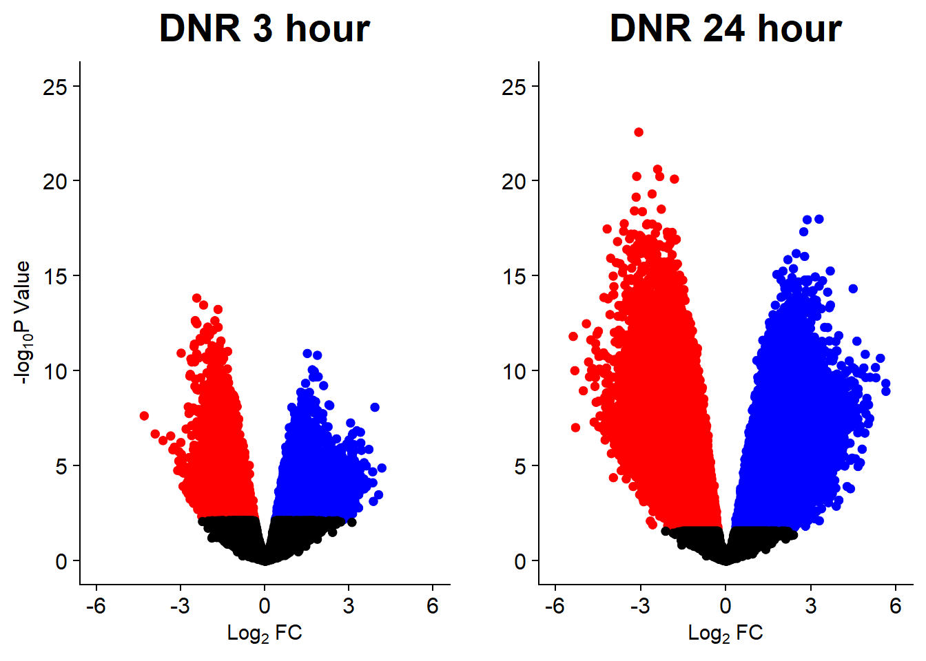

Past versions of "Volcano plots-1.png"

Version	Author	Date
cf05574	reneeisnowhere	2025-05-14
fee3875	reneeisnowhere	2025-05-06

plot_grid(v3,v4,  rel_widths =c(1,1))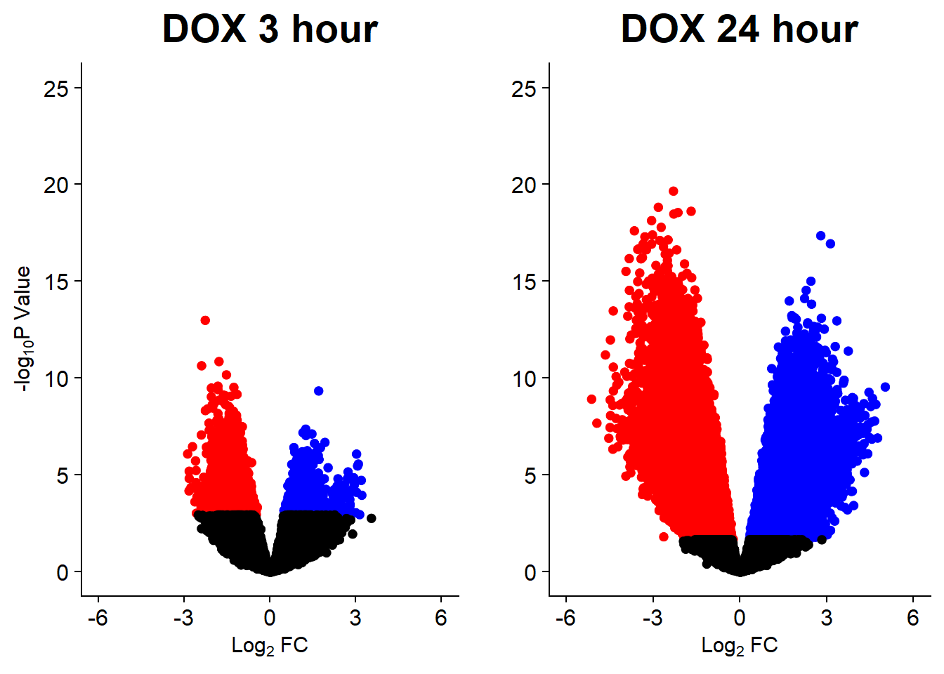

Past versions of "Volcano plots-2.png"

Version	Author	Date
cf05574	reneeisnowhere	2025-05-14
fee3875	reneeisnowhere	2025-05-06

plot_grid(v5,v6,  rel_widths =c(1,1))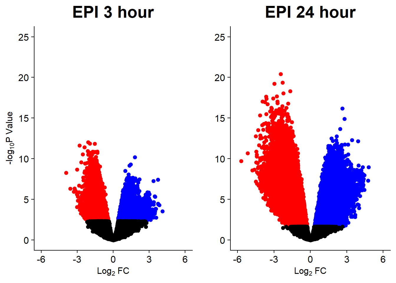

Past versions of "Volcano plots-3.png"

Version	Author	Date
cf05574	reneeisnowhere	2025-05-14
fee3875	reneeisnowhere	2025-05-06

plot_grid(v7,v8,  rel_widths =c(1,1))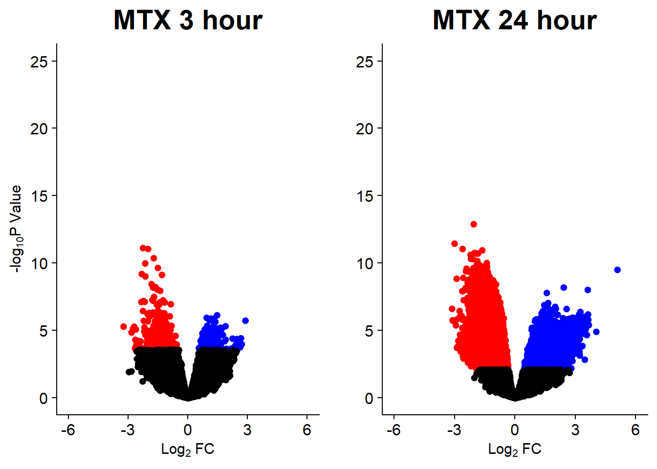

Past versions of "Volcano plots-4.png"

Version	Author	Date
cf05574	reneeisnowhere	2025-05-14
fee3875	reneeisnowhere	2025-05-06

plot_grid(v9,v10,  rel_widths =c(1,1))

Past versions of "Volcano plots-5.png"

Version	Author	Date
cf05574	reneeisnowhere	2025-05-14
fee3875	reneeisnowhere	2025-05-06

Making the median dataframes by time. The files were saved as .csv for future use.

all_results <- bind_rows(save_list, .id = "group")

median_df <- all_results %>% 
  separate(group, into=c("trt","time"),sep = "_") %>% 
  pivot_wider(., id_cols=c(time,genes), names_from = trt, values_from = logFC) %>% 
  rowwise() %>% 
  mutate(median_ATAC_lfc= median(c_across(DNR:TRZ)))

median_3_lfc <-   median_df %>%
    dplyr::filter(time == "3") %>% 
  ungroup() %>% 
  dplyr::select(time, genes,median_ATAC_lfc) %>% 
  dplyr::rename("med_3h_lfc"=median_ATAC_lfc, "peak"=genes)
  

median_24_lfc <- median_df %>%
    dplyr::filter(time == "24") %>% 
  ungroup() %>% 
  dplyr::select(time, genes,median_ATAC_lfc) %>% 
  dplyr::rename("med_24h_lfc"=median_ATAC_lfc,, "peak"=genes)
  
write_csv(median_3_lfc, "data/Final_four_data/re_analysis/median_3_lfc_norm.csv")
write_csv(median_24_lfc, "data/Final_four_data/re_analysis/median_24_lfc_norm.csv")

Correlation of LFC between treatments

FCmatrix_ff <- subset(efit2$coefficients)

colnames(FCmatrix_ff) <-
  c("DNR\n3h",
    "DOX\n3h",
    "EPI\n3h",
    "MTX\n3h",
    "TRZ\n3h",
    "DNR\n24h",
    "DOX\n24h",
    "EPI\n24h",
    "MTX\n24h",
    "TRZ\n24h"
     )


mat_col_ff <-
  data.frame(
    time = c(rep("3 hours", 5), rep("24 hours", 5)),
    class = (c(
      "AC", "AC", "AC", "nAC","nAC",  "AC", "AC", "AC", "nAC","nAC" 
    )))
rownames(mat_col_ff) <- colnames(FCmatrix_ff)

mat_colors_ff <-
  list(
    time = c("pink", "chocolate4"),
    class = c("yellow1", "lightgreen"))

names(mat_colors_ff$time) <- unique(mat_col_ff$time)
names(mat_colors_ff$class) <- unique(mat_col_ff$class)
# names(mat_colors_FC$TOP2i) <- unique(mat_col_FC$TOP2i)
corrFC_ff <- cor(FCmatrix_ff)

htanno_ff <-  HeatmapAnnotation(df = mat_col_ff, col = mat_colors_ff)
Heatmap(corrFC_ff, top_annotation = htanno_ff)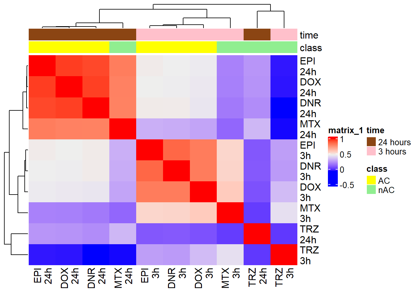

Past versions of "LFC correlation-1.png"

Version	Author	Date
5e6e462	reneeisnowhere	2025-05-07

drug_pal <- c("#8B006D","#DF707E","#F1B72B", "#3386DD","#707031","#41B333")

# all_results <- bind_rows(save_list, .id = "group")
DNR_3_top3_ff <- row.names(V.DNR_3.top[1:3,])

log_filt_ff <-
  filt_raw_counts_noY %>% 
   cpm(., log=TRUE)%>%
  as.data.frame() 
  
row.names(log_filt_ff) <- row.names(filt_raw_counts_noY)

log_filt_ff %>% 
  dplyr::filter(row.names(.) %in% DNR_3_top3_ff) %>% 
  mutate(Peak = row.names(.)) %>% 
  pivot_longer(cols = !Peak, names_to = "sample", values_to = "counts") %>% 
  separate("sample", into = c("indv","trt","time")) %>% 
  mutate(time=factor(time, levels = c("3h","24h"))) %>% 
  mutate(trt=factor(trt, levels= c("DOX","EPI","DNR","MTX","TRZ","VEH"))) %>% 
  ggplot(., aes (x = time, y=counts))+
  geom_boxplot(aes(fill=trt))+
  facet_wrap(Peak~.)+
  ggtitle("top 3 DAR in 3 hour DNR")+
  scale_fill_manual(values = drug_pal)+
  theme_bw()

Past versions of "example 3hr accesibility-1.png"

Version	Author	Date
4163890	reneeisnowhere	2025-05-12

DOX_3_top3_ff <- row.names(V.DOX_3.top[1:3,])

log_filt_ff %>% 
  dplyr::filter(row.names(.) %in% DOX_3_top3_ff) %>% 
  mutate(Peak = row.names(.)) %>% 
  pivot_longer(cols = !Peak, names_to = "sample", values_to = "counts") %>% 
  separate("sample", into = c("indv","trt","time")) %>% 
  mutate(time=factor(time, levels = c("3h","24h"))) %>% 
  mutate(trt=factor(trt, levels= c("DOX","EPI","DNR","MTX","TRZ","VEH"))) %>% 
  ggplot(., aes (x = time, y=counts))+
  geom_boxplot(aes(fill=trt))+
  facet_wrap(Peak~.)+
  ggtitle("top 3 DAR in 3 hour DOX")+
  scale_fill_manual(values = drug_pal)+
  theme_bw()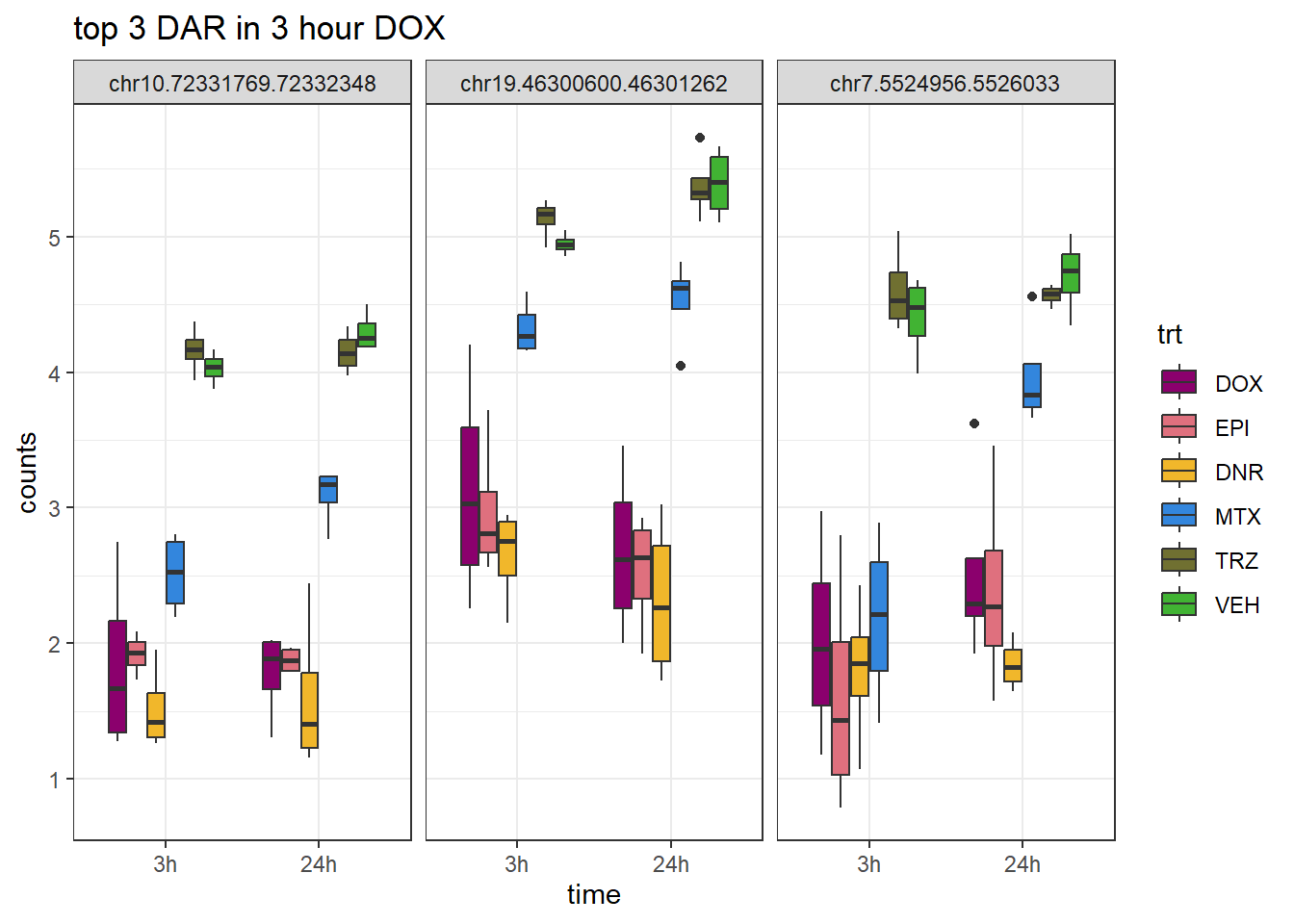

Past versions of "example 3hr accesibility-2.png"

Version	Author	Date
4163890	reneeisnowhere	2025-05-12

EPI_3_top3_ff <- row.names(V.EPI_3.top[1:3,])

log_filt_ff %>% 
  dplyr::filter(row.names(.) %in% EPI_3_top3_ff) %>% 
  mutate(Peak = row.names(.)) %>% 
  pivot_longer(cols = !Peak, names_to = "sample", values_to = "counts") %>% 
  separate("sample", into = c("indv","trt","time")) %>% 
  mutate(time=factor(time, levels = c("3h","24h"))) %>% 
  mutate(trt=factor(trt, levels= c("DOX","EPI","DNR","MTX","TRZ","VEH"))) %>% 
  ggplot(., aes (x = time, y=counts))+
  geom_boxplot(aes(fill=trt))+
  facet_wrap(Peak~.)+
  ggtitle("top 3 DAR in 3 hour EPI")+
  scale_fill_manual(values = drug_pal)+
  theme_bw()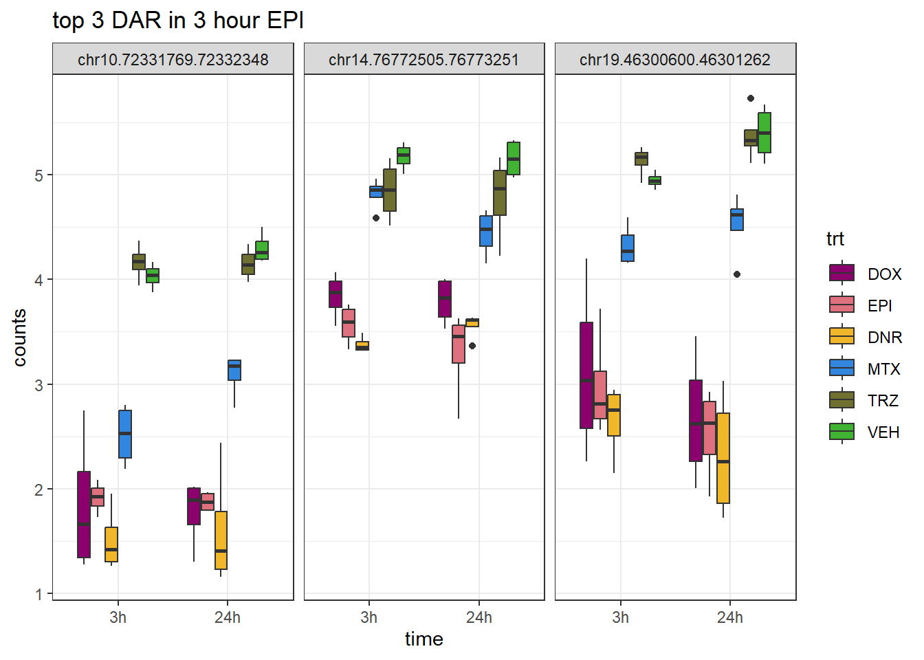

Past versions of "example 3hr accesibility-3.png"

Version	Author	Date
4163890	reneeisnowhere	2025-05-12

MTX_3_top3_ff <- row.names(V.MTX_3.top[1:3,])

log_filt_ff %>% 
  dplyr::filter(row.names(.) %in% MTX_3_top3_ff) %>% 
  mutate(Peak = row.names(.)) %>% 
  pivot_longer(cols = !Peak, names_to = "sample", values_to = "counts") %>% 
  separate("sample", into = c("indv","trt","time")) %>% 
  mutate(time=factor(time, levels = c("3h","24h"))) %>% 
  mutate(trt=factor(trt, levels= c("DOX","EPI","DNR","MTX","TRZ","VEH"))) %>% 
  ggplot(., aes (x = time, y=counts))+
  geom_boxplot(aes(fill=trt))+
  facet_wrap(Peak~.)+
  ggtitle("top 3 DAR in 3 hour MTX")+
  scale_fill_manual(values = drug_pal)+
  theme_bw()

Past versions of "example 3hr accesibility-4.png"

Version	Author	Date
4163890	reneeisnowhere	2025-05-12

TRZ_3_top3_ff <- row.names(V.TRZ_3.top[1:3,])

log_filt_ff %>% 
  dplyr::filter(row.names(.) %in% TRZ_3_top3_ff) %>% 
  mutate(Peak = row.names(.)) %>% 
  pivot_longer(cols = !Peak, names_to = "sample", values_to = "counts") %>% 
  separate("sample", into = c("indv","trt","time")) %>% 
  mutate(time=factor(time, levels = c("3h","24h"))) %>% 
  mutate(trt=factor(trt, levels= c("DOX","EPI","DNR","MTX","TRZ","VEH"))) %>% 
  ggplot(., aes (x = time, y=counts))+
  geom_boxplot(aes(fill=trt))+
  facet_wrap(Peak~.)+
  ggtitle("top 3 DAR in 3 hour TRZ")+
 scale_fill_manual(values = drug_pal)+
  theme_bw()

Past versions of "example 3hr accesibility-5.png"

Version	Author	Date
4163890	reneeisnowhere	2025-05-12

DNR_24_top3_ff <- row.names(V.DNR_24.top[1:3,])


log_filt_ff %>% 
  dplyr::filter(row.names(.) %in% DNR_24_top3_ff) %>% 
  mutate(Peak = row.names(.)) %>% 
  pivot_longer(cols = !Peak, names_to = "sample", values_to = "counts") %>% 
  separate("sample", into = c("indv","trt","time")) %>% 
  mutate(time=factor(time, levels = c("3h","24h"))) %>% 
  mutate(trt=factor(trt, levels= c("DOX","EPI","DNR","MTX","TRZ","VEH"))) %>% 
  ggplot(., aes (x = time, y=counts))+
  geom_boxplot(aes(fill=trt))+
  facet_wrap(Peak~.)+
  ggtitle("top 3 DAR in 24 hour DNR")+
  scale_fill_manual(values = drug_pal)+
  theme_bw()

Past versions of "example 24hr accesibility-1.png"

Version	Author	Date
4163890	reneeisnowhere	2025-05-12

DOX_24_top3_ff <- row.names(V.DOX_24.top[1:3,])

log_filt_ff %>% 
  dplyr::filter(row.names(.) %in% DOX_24_top3_ff) %>% 
  mutate(Peak = row.names(.)) %>% 
  pivot_longer(cols = !Peak, names_to = "sample", values_to = "counts") %>% 
  separate("sample", into = c("indv","trt","time")) %>% 
  mutate(time=factor(time, levels = c("3h","24h"))) %>% 
  mutate(trt=factor(trt, levels= c("DOX","EPI","DNR","MTX","TRZ","VEH"))) %>% 
  ggplot(., aes (x = time, y=counts))+
  geom_boxplot(aes(fill=trt))+
  facet_wrap(Peak~.)+
  ggtitle("top 3 DAR in 24 hour DOX")+
  scale_fill_manual(values = drug_pal)+
  theme_bw()

Past versions of "example 24hr accesibility-2.png"

Version	Author	Date
4163890	reneeisnowhere	2025-05-12

EPI_24_top3_ff <- row.names(V.EPI_24.top[1:3,])

log_filt_ff %>% 
  dplyr::filter(row.names(.) %in% EPI_24_top3_ff) %>% 
  mutate(Peak = row.names(.)) %>% 
  pivot_longer(cols = !Peak, names_to = "sample", values_to = "counts") %>% 
  separate("sample", into = c("indv","trt","time")) %>% 
  mutate(time=factor(time, levels = c("3h","24h"))) %>% 
  mutate(trt=factor(trt, levels= c("DOX","EPI","DNR","MTX","TRZ","VEH"))) %>% 
  ggplot(., aes (x = time, y=counts))+
  geom_boxplot(aes(fill=trt))+
  facet_wrap(Peak~.)+
  ggtitle("top 3 DAR in 24 hour EPI")+
  scale_fill_manual(values = drug_pal)+
  theme_bw()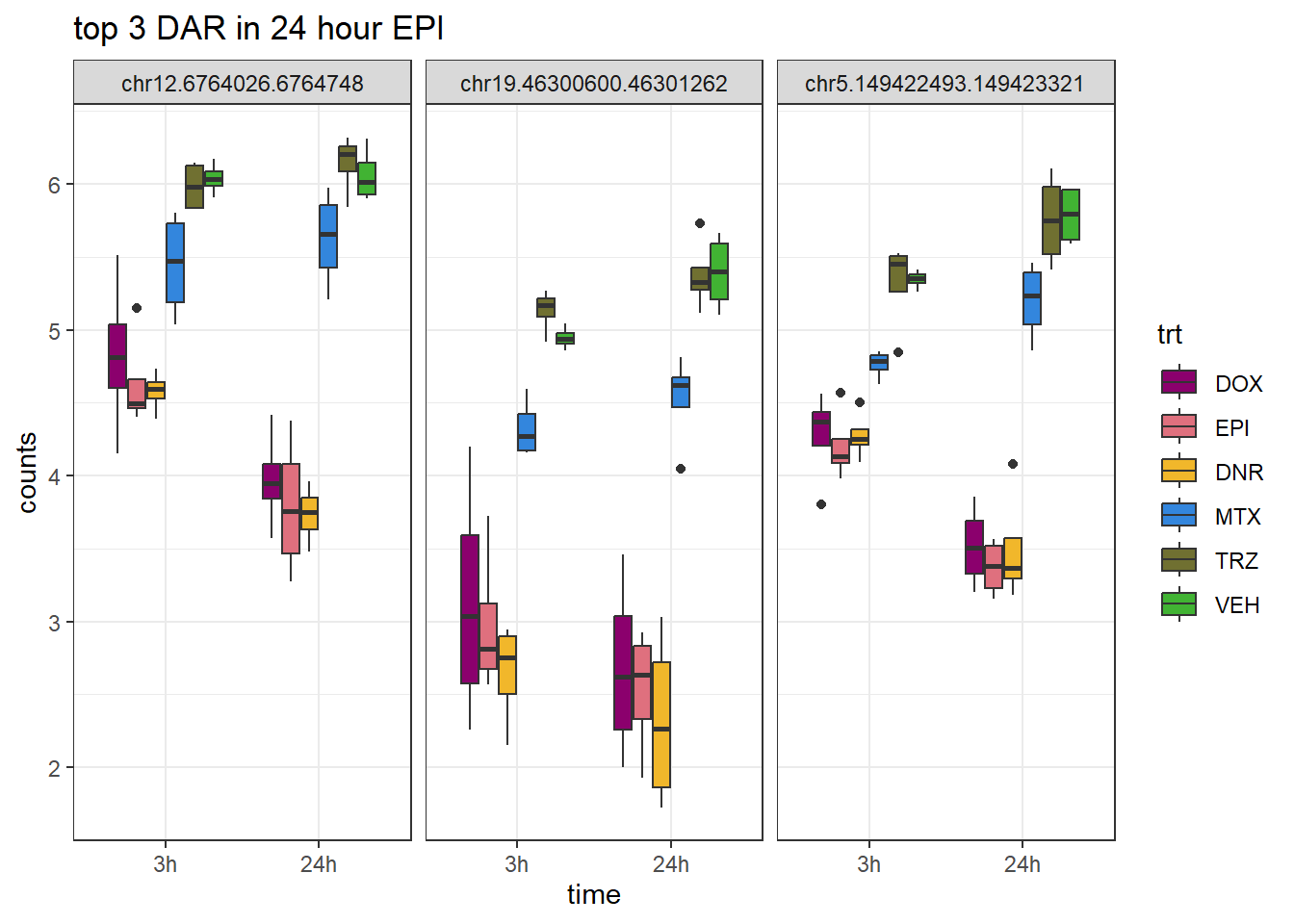

Past versions of "example 24hr accesibility-3.png"

Version	Author	Date
4163890	reneeisnowhere	2025-05-12

MTX_24_top3_ff <- row.names(V.MTX_24.top[1:3,])

log_filt_ff %>% 
  dplyr::filter(row.names(.) %in% MTX_24_top3_ff) %>% 
  mutate(Peak = row.names(.)) %>% 
  pivot_longer(cols = !Peak, names_to = "sample", values_to = "counts") %>% 
  separate("sample", into = c("indv","trt","time")) %>% 
  mutate(time=factor(time, levels = c("3h","24h"))) %>% 
  mutate(trt=factor(trt, levels= c("DOX","EPI","DNR","MTX","TRZ","VEH"))) %>% 
  ggplot(., aes (x = time, y=counts))+
  geom_boxplot(aes(fill=trt))+
  facet_wrap(Peak~.)+
  ggtitle("top 3 DAR in 24 hour MTX")+
  scale_fill_manual(values = drug_pal)+
  theme_bw()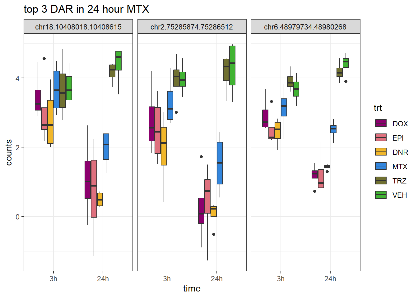

Past versions of "example 24hr accesibility-4.png"

Version	Author	Date
4163890	reneeisnowhere	2025-05-12

TRZ_24_top3_ff <- row.names(V.TRZ_24.top[1:3,])

log_filt_ff %>% 
  dplyr::filter(row.names(.) %in% TRZ_24_top3_ff) %>% 
  mutate(Peak = row.names(.)) %>% 
  pivot_longer(cols = !Peak, names_to = "sample", values_to = "counts") %>% 
  separate("sample", into = c("indv","trt","time")) %>% 
  mutate(time=factor(time, levels = c("3h","24h"))) %>% 
  mutate(trt=factor(trt, levels= c("DOX","EPI","DNR","MTX","TRZ","VEH"))) %>% 
  ggplot(., aes (x = time, y=counts))+
  geom_boxplot(aes(fill=trt))+
  facet_wrap(Peak~.)+
  ggtitle("top 3 DAR in 24 hour TRZ")+
  scale_fill_manual(values = drug_pal)+
  theme_bw()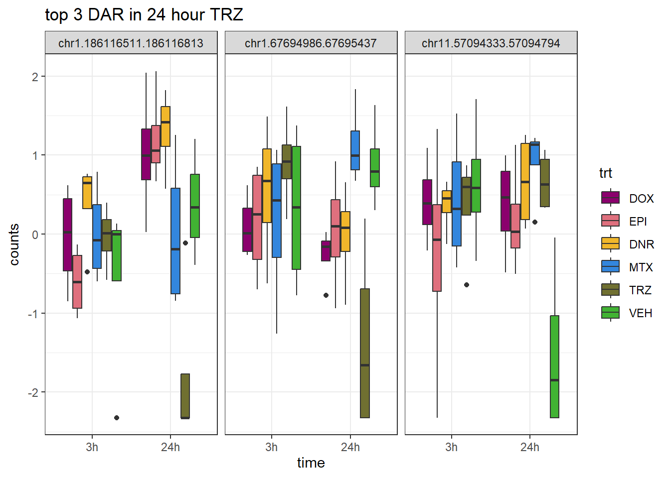

Past versions of "example 24hr accesibility-5.png"

Version	Author	Date
4163890	reneeisnowhere	2025-05-12

Examining around the adj. p value cutoff

DNR_closest <-  V.DNR_3.top %>%
  dplyr::filter(adj.P.Val<0.05) %>% 
  slice_tail(n=5)


log_filt_ff %>% 
  dplyr::filter(row.names(.) %in% DNR_closest$genes) %>% 
  mutate(Peak = row.names(.)) %>% 
  pivot_longer(cols = !Peak, names_to = "sample", values_to = "counts") %>% 
  separate("sample", into = c("indv","trt","time")) %>% 
  mutate(time=factor(time, levels = c("3h","24h"))) %>% 
  mutate(trt=factor(trt, levels= c("DOX","EPI","DNR","MTX","TRZ","VEH"))) %>% 
  ggplot(., aes (x = time, y=counts))+
  geom_boxplot(aes(fill=trt))+
  facet_wrap(Peak~.)+
  ggtitle("Bottom DAR in 3 hour DNR")+
  scale_fill_manual(values = drug_pal)+
  theme_bw()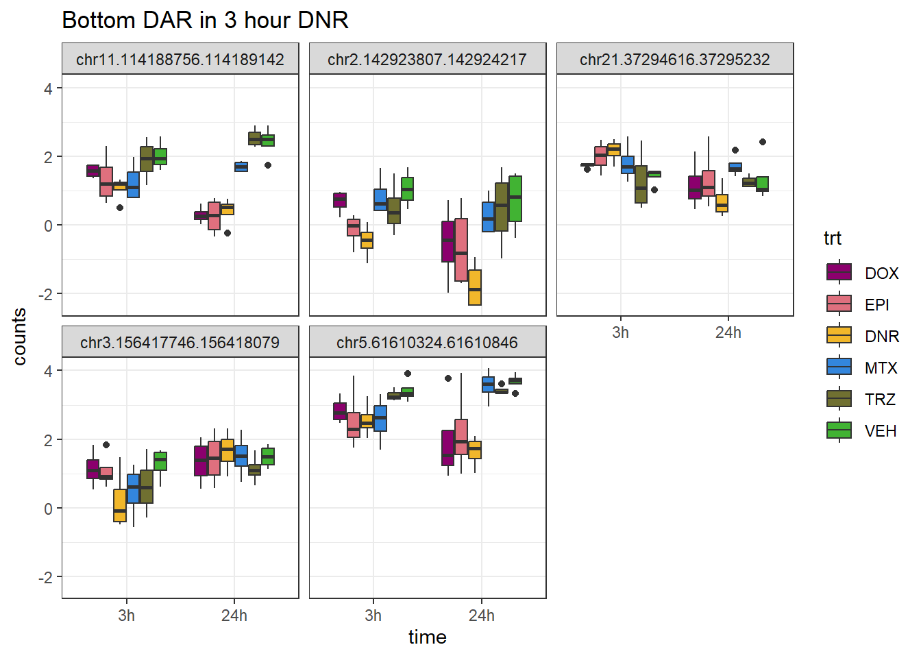

Past versions of "bottom slices 3 hour-1.png"

Version	Author	Date
f0c5b69	reneeisnowhere	2025-06-05

DOX_closest <-  V.DOX_3.top %>%
  dplyr::filter(adj.P.Val<0.05) %>% 
  slice_tail(n=5)

log_filt_ff %>% 
  dplyr::filter(row.names(.) %in% DOX_closest$genes) %>% 
  mutate(Peak = row.names(.)) %>% 
  pivot_longer(cols = !Peak, names_to = "sample", values_to = "counts") %>% 
  separate("sample", into = c("indv","trt","time")) %>% 
  mutate(time=factor(time, levels = c("3h","24h"))) %>% 
  mutate(trt=factor(trt, levels= c("DOX","EPI","DNR","MTX","TRZ","VEH"))) %>% 
  ggplot(., aes (x = time, y=counts))+
  geom_boxplot(aes(fill=trt))+
  facet_wrap(Peak~.)+
  ggtitle("bottom 5 DAR in 3 hour DOX")+
  scale_fill_manual(values = drug_pal)+
  theme_bw()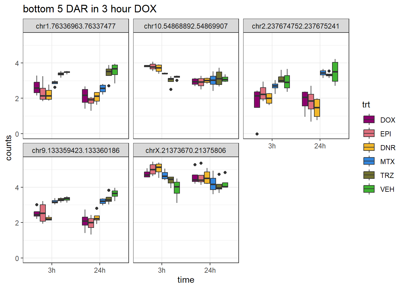

Past versions of "bottom slices 3 hour-2.png"

Version	Author	Date
f0c5b69	reneeisnowhere	2025-06-05

EPI_closest <-  V.EPI_3.top %>%
  dplyr::filter(adj.P.Val<0.05) %>% 
  slice_tail(n=5)

log_filt_ff %>% 
  dplyr::filter(row.names(.) %in% EPI_closest$genes) %>% 
  mutate(Peak = row.names(.)) %>% 
  pivot_longer(cols = !Peak, names_to = "sample", values_to = "counts") %>% 
  separate("sample", into = c("indv","trt","time")) %>% 
  mutate(time=factor(time, levels = c("3h","24h"))) %>% 
  mutate(trt=factor(trt, levels= c("DOX","EPI","DNR","MTX","TRZ","VEH"))) %>% 
  ggplot(., aes (x = time, y=counts))+
  geom_boxplot(aes(fill=trt))+
  facet_wrap(Peak~.)+
  ggtitle("bottom 5 DAR in 3 hour EPI")+
  scale_fill_manual(values = drug_pal)+
  theme_bw()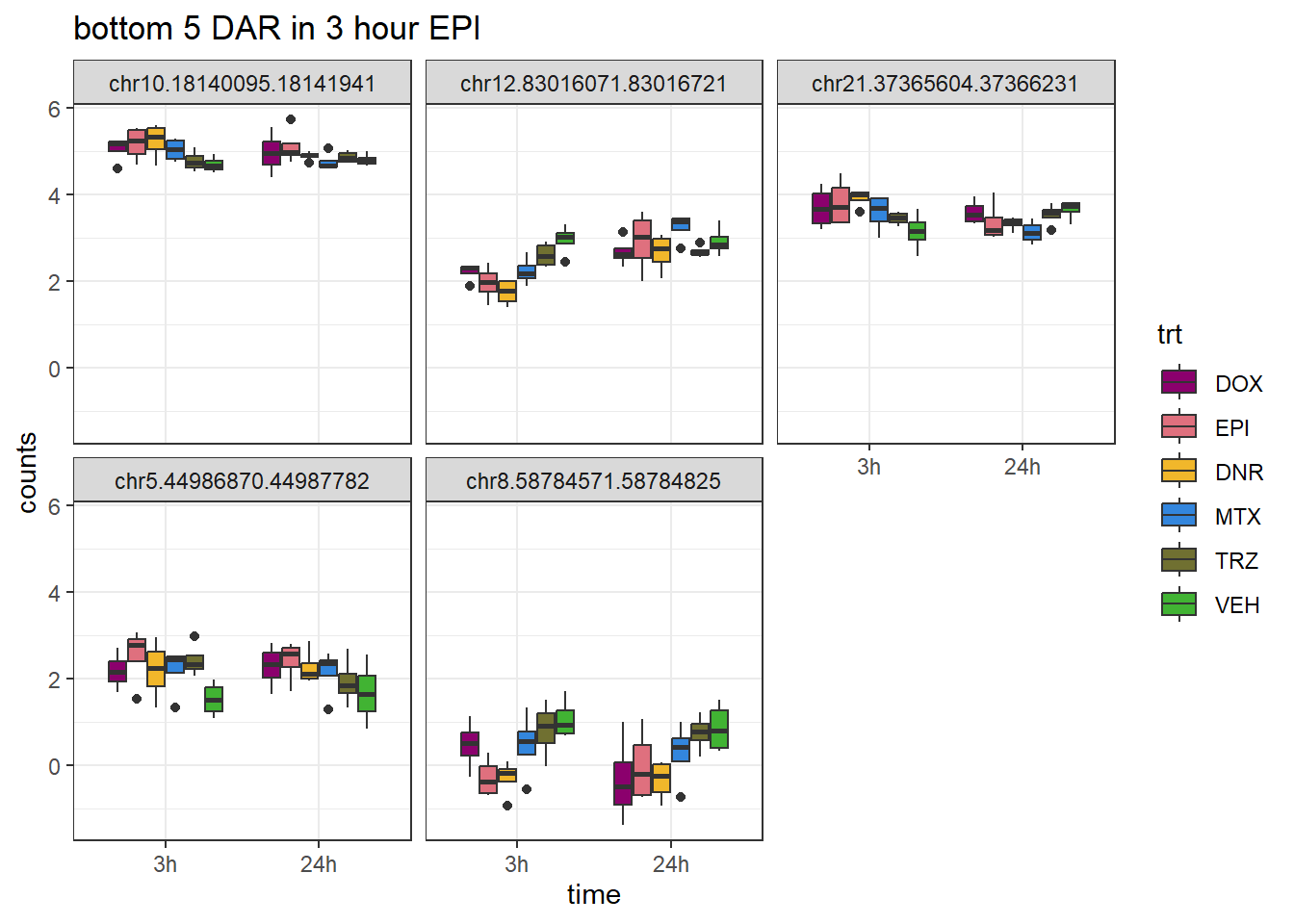

Past versions of "bottom slices 3 hour-3.png"

Version	Author	Date
f0c5b69	reneeisnowhere	2025-06-05

MTX_closest <-  V.MTX_3.top %>%
  dplyr::filter(adj.P.Val<0.05) %>% 
  slice_tail(n=5)

log_filt_ff %>% 
  dplyr::filter(row.names(.) %in% MTX_closest$genes) %>% 
  mutate(Peak = row.names(.)) %>% 
  pivot_longer(cols = !Peak, names_to = "sample", values_to = "counts") %>% 
  separate("sample", into = c("indv","trt","time")) %>% 
  mutate(time=factor(time, levels = c("3h","24h"))) %>% 
  mutate(trt=factor(trt, levels= c("DOX","EPI","DNR","MTX","TRZ","VEH"))) %>% 
  ggplot(., aes (x = time, y=counts))+
  geom_boxplot(aes(fill=trt))+
  facet_wrap(Peak~.)+
  ggtitle("bottom 5 DAR in 3 hour MTX")+
  scale_fill_manual(values = drug_pal)+
  theme_bw()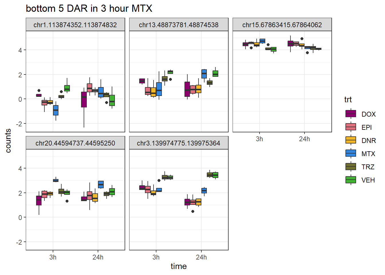

Past versions of "bottom slices 3 hour-4.png"

Version	Author	Date
f0c5b69	reneeisnowhere	2025-06-05

TRZ_closest <-  V.TRZ_3.top %>%
  dplyr::filter(adj.P.Val<0.05) %>% 
  slice_tail(n=5)

log_filt_ff %>% 
  dplyr::filter(row.names(.) %in% TRZ_closest$genes) %>% 
  mutate(Peak = row.names(.)) %>% 
  pivot_longer(cols = !Peak, names_to = "sample", values_to = "counts") %>% 
  separate("sample", into = c("indv","trt","time")) %>% 
  mutate(time=factor(time, levels = c("3h","24h"))) %>% 
  mutate(trt=factor(trt, levels= c("DOX","EPI","DNR","MTX","TRZ","VEH"))) %>% 
  ggplot(., aes (x = time, y=counts))+
  geom_boxplot(aes(fill=trt))+
  facet_wrap(Peak~.)+
  ggtitle("bottom 5 DAR in 3 hour TRZ")+
  scale_fill_manual(values = drug_pal)+
  theme_bw()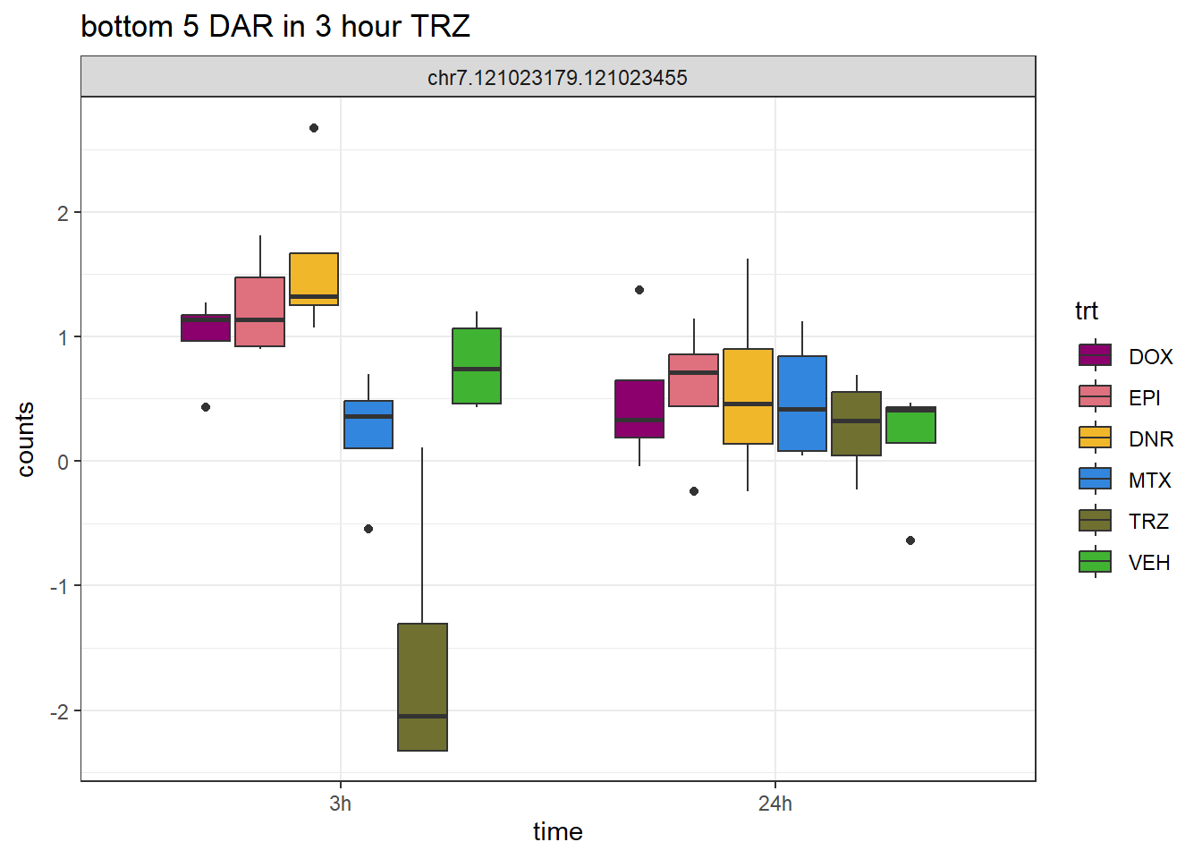

Past versions of "bottom slices 3 hour-5.png"

Version	Author	Date
f0c5b69	reneeisnowhere	2025-06-05

DNR_closest <-  V.DNR_24.top %>%
  dplyr::filter(adj.P.Val<0.05) %>% 
  slice_tail(n=5)


log_filt_ff %>% 
  dplyr::filter(row.names(.) %in% DNR_closest$genes) %>% 
  mutate(Peak = row.names(.)) %>% 
  pivot_longer(cols = !Peak, names_to = "sample", values_to = "counts") %>% 
  separate("sample", into = c("indv","trt","time")) %>% 
  mutate(time=factor(time, levels = c("3h","24h"))) %>% 
  mutate(trt=factor(trt, levels= c("DOX","EPI","DNR","MTX","TRZ","VEH"))) %>% 
  ggplot(., aes (x = time, y=counts))+
  geom_boxplot(aes(fill=trt))+
  facet_wrap(Peak~.)+
  ggtitle("Bottom DAR in 24 hour DNR")+
  scale_fill_manual(values = drug_pal)+
  theme_bw()

Past versions of "bottom slices 24 hour-1.png"

Version	Author	Date
f0c5b69	reneeisnowhere	2025-06-05

DOX_closest <-  V.DOX_24.top %>%
  dplyr::filter(adj.P.Val<0.05) %>% 
  slice_tail(n=5)

log_filt_ff %>% 
  dplyr::filter(row.names(.) %in% DOX_closest$genes) %>% 
  mutate(Peak = row.names(.)) %>% 
  pivot_longer(cols = !Peak, names_to = "sample", values_to = "counts") %>% 
  separate("sample", into = c("indv","trt","time")) %>% 
  mutate(time=factor(time, levels = c("3h","24h"))) %>% 
  mutate(trt=factor(trt, levels= c("DOX","EPI","DNR","MTX","TRZ","VEH"))) %>% 
  ggplot(., aes (x = time, y=counts))+
  geom_boxplot(aes(fill=trt))+
  facet_wrap(Peak~.)+
  ggtitle("bottom 5 DAR in 24 hour DOX")+
  scale_fill_manual(values = drug_pal)+
  theme_bw()

Past versions of "bottom slices 24 hour-2.png"

Version	Author	Date
f0c5b69	reneeisnowhere	2025-06-05

EPI_closest <-  V.EPI_24.top %>%
  dplyr::filter(adj.P.Val<0.05) %>% 
  slice_tail(n=5)

log_filt_ff %>% 
  dplyr::filter(row.names(.) %in% EPI_closest$genes) %>% 
  mutate(Peak = row.names(.)) %>% 
  pivot_longer(cols = !Peak, names_to = "sample", values_to = "counts") %>% 
  separate("sample", into = c("indv","trt","time")) %>% 
  mutate(time=factor(time, levels = c("3h","24h"))) %>% 
  mutate(trt=factor(trt, levels= c("DOX","EPI","DNR","MTX","TRZ","VEH"))) %>% 
  ggplot(., aes (x = time, y=counts))+
  geom_boxplot(aes(fill=trt))+
  facet_wrap(Peak~.)+
  ggtitle("bottom 5 DAR in 24 hour EPI")+
  scale_fill_manual(values = drug_pal)+
  theme_bw()

Past versions of "bottom slices 24 hour-3.png"

Version	Author	Date
f0c5b69	reneeisnowhere	2025-06-05

MTX_closest <-  V.MTX_24.top %>%
  dplyr::filter(adj.P.Val<0.05) %>% 
  slice_tail(n=5)

log_filt_ff %>% 
  dplyr::filter(row.names(.) %in% MTX_closest$genes) %>% 
  mutate(Peak = row.names(.)) %>% 
  pivot_longer(cols = !Peak, names_to = "sample", values_to = "counts") %>% 
  separate("sample", into = c("indv","trt","time")) %>% 
  mutate(time=factor(time, levels = c("3h","24h"))) %>% 
  mutate(trt=factor(trt, levels= c("DOX","EPI","DNR","MTX","TRZ","VEH"))) %>% 
  ggplot(., aes (x = time, y=counts))+
  geom_boxplot(aes(fill=trt))+
  facet_wrap(Peak~.)+
  ggtitle("bottom 5 DAR in 24 hour MTX")+
  scale_fill_manual(values = drug_pal)+
  theme_bw()

Past versions of "bottom slices 24 hour-4.png"

Version	Author	Date
f0c5b69	reneeisnowhere	2025-06-05

# TRZ_closest <-  V.TRZ_24.top %>%
#   dplyr::filter(adj.P.Val<0.05) %>% 
#   slice_tail(n=5)
# 
# log_filt_ff %>% 
#   dplyr::filter(row.names(.) %in% TRZ_closest$genes) %>% 
#   mutate(Peak = row.names(.)) %>% 
#   pivot_longer(cols = !Peak, names_to = "sample", values_to = "counts") %>% 
#   separate("sample", into = c("indv","trt","time")) %>% 
#   mutate(time=factor(time, levels = c("3h","24h"))) %>% 
#   mutate(trt=factor(trt, levels= c("DOX","EPI","DNR","MTX","TRZ","VEH"))) %>% 
#   ggplot(., aes (x = time, y=counts))+
#   geom_boxplot(aes(fill=trt))+
#   facet_wrap(Peak~.)+
#   ggtitle("bottom 5 DAR in 24 hour TRZ")+
#   scale_fill_manual(values = drug_pal)+
#   theme_bw()

toptable_results <- readRDS("data/Final_four_data/re_analysis/Toptable_results.RDS")
library(openxlsx)
output_dir <- "data/Final_four_data/re_analysis/ATAC_excel_outputs"

# Create directory if it doesn't exist
if (!dir.exists(output_dir)) {
  dir.create(output_dir, recursive = TRUE)
}

# Export each data frame to a separate .xlsx file
for (name in names(toptable_results)) {
  # Create a new workbook
  wb <- createWorkbook()
  
  # Add a worksheet (you can use the name as the sheet name too)
  addWorksheet(wb, name)
  
  # Write the data frame to the sheet
  writeData(wb, sheet = name, toptable_results[[name]])
  # Full file path using file.path()
  output_file <- file.path(output_dir, paste0(name, ".xlsx"))
  saveWorkbook(wb, file = output_file, overwrite = TRUE)
}

Extracting top DARs

toptable_results <- readRDS("data/Final_four_data/re_analysis/Toptable_results.RDS")

all_results  <- toptable_results %>%
  imap(~ .x %>% tibble::rownames_to_column(var = "rowname") %>%
         mutate(source = .y)) %>%
  bind_rows()
all_results_list  <- toptable_results %>%
  imap(~ .x %>% tibble::rownames_to_column(var = "rowname") %>%
         mutate(source = .y)) 

sig_meta_and_loc <- all_results %>% 
  dplyr::filter(adj.P.Val<0.05) %>%  ## filter by pvalue
##Create parsed dataframe from "rowname" column, "genes column will keep id"
   separate(rowname, into = c("seqnames", "start", "end"), sep = "\\.", convert = TRUE)
###split into lists by DNR_3, etc..
sig_meta_and_loc_split <- split(sig_meta_and_loc, sig_meta_and_loc$source)
### Convert to Granges for downstream
sig_meta_and_loc_split_gr <- lapply(sig_meta_and_loc_split, function(sub_df) {
  GRanges(
    seqnames = sub_df$seqnames,
    ranges = IRanges(start = sub_df$start, end = sub_df$end),
    mcols = sub_df %>% dplyr::select(-seqnames, -start, -end)
  )
})


notsig_meta_and_loc <- all_results %>% 
  dplyr::filter(adj.P.Val>0.05) %>% 
  separate(rowname, into = c("seqnames","start","end"), sep = "\\.", convert=TRUE)
    
notsig_meta_and_loc_split <- split(notsig_meta_and_loc, notsig_meta_and_loc$source)

notsig_meta_and_loc_split_gr <- lapply(notsig_meta_and_loc_split, function(sub_df) {
  GRanges(
    seqnames = sub_df$seqnames,
    ranges = IRanges(start = sub_df$start, end = sub_df$end),
    mcols = sub_df %>% dplyr::select(-seqnames, -start, -end)
  )
})

all_DAR_regions <- all_results %>% 
   separate(rowname, into = c("seqnames", "start", "end"), sep = "\\.", convert = TRUE)
all_DAR_regions_list <- split(all_DAR_regions, all_DAR_regions$source)

all_DAR_regions_gr <- lapply(all_DAR_regions_list, function(sub_df) {
  GRanges(
    seqnames = sub_df$seqnames,
    ranges = IRanges(start = sub_df$start, end = sub_df$end),
    mcols = sub_df %>% dplyr::select(-seqnames, -start, -end)
  )
})

# Folder with input BED files

output_dir <- "data/Final_four_data/re_analysis/motif_beds_centered"

# Create output folder if needed
dir.create(output_dir, showWarnings = FALSE)

# Loop through each BED file
for (name in names(sig_meta_and_loc_split_gr)) {
  gr <- sig_meta_and_loc_split_gr[[name]]
  
  # Recenter each region to 200 bp around its midpoint
  gr_centered <- resize(gr, width = 200, fix = "center")
  
  # Export to BED (auto converts to 0-based)
  export(gr_centered, con = file.path(output_dir, paste0(name, "sig_centered.bed")), format = "BED")
}


### not significant DAR regions for xstreme

for (name in names(notsig_meta_and_loc_split_gr)) {
  gr <- notsig_meta_and_loc_split_gr[[name]]
  
  # Recenter each region to 200 bp around its midpoint
  gr_centered <- resize(gr, width = 200, fix = "center")
  
  # Export to BED (auto converts to 0-based)
  export(gr_centered, con = file.path(output_dir, paste0(name, "notsig_centered.bed")), format = "BED")
}

Examining regions between sig DARs and trt_time

sig_venn_list <- sapply(sig_meta_and_loc_split, function(x) x$genes)
sig_venn_3hr <- sig_venn_list[c("DOX_3","EPI_3", "DNR_3","MTX_3")]
sig_venn_24hr <- sig_venn_list[c("DOX_24","EPI_24", "DNR_24","MTX_24")]

sig_3hr_df <- dplyr::bind_rows(
  lapply(names(sig_venn_3hr), function(name) {
    data.frame(gene = sig_venn_3hr[[name]], condition = name)
  })
) %>% 
  distinct(gene)
sig_24hr_df <- dplyr::bind_rows(
  lapply(names(sig_venn_24hr), function(name) {
    data.frame(gene = sig_venn_24hr[[name]], condition = name)
  })
) %>% 
  distinct(gene)

ggVennDiagram(list("3hr_regions"=sig_3hr_df$gene,"24hr_regions"=sig_24hr_df$gene))+
   xlim(-5, 5)+
  coord_flip()

Past versions of "DAR venn-1.png"

Version	Author	Date
30dc0d7	reneeisnowhere	2025-07-21
f0c5b69	reneeisnowhere	2025-06-05

ggVennDiagram::ggVennDiagram(sig_venn_3hr)

Past versions of "DAR venn-2.png"

Version	Author	Date
30dc0d7	reneeisnowhere	2025-07-21
f0c5b69	reneeisnowhere	2025-06-05

ggVennDiagram::ggVennDiagram(sig_venn_24hr)

Past versions of "DAR venn-3.png"

Version	Author	Date
30dc0d7	reneeisnowhere	2025-07-21

saveRDS(sig_meta_and_loc_split,"Sig_meta")


sig_3hr_obj <- ggVennDiagram::Venn(sig_venn_list[c("DOX_3","EPI_3", "DNR_3","MTX_3")])
sig_24hr_obj <- ggVennDiagram::Venn(sig_venn_list[c("DOX_24","EPI_24", "DNR_24","MTX_24")])
sig_3hr_obj <- ggVennDiagram::process_data(sig_3hr_obj)
sig_24hr_obj <- ggVennDiagram::process_data(sig_24hr_obj)

sig_3hr_regions <- ggVennDiagram::venn_region(sig_3hr_obj)
sig_24hr_regions<- ggVennDiagram::venn_region(sig_24hr_obj)
sig_3hr_shared <- sig_3hr_obj$regionLabel$item[[11]]
sig_24hr_shared <-   sig_24hr_obj$regionLabel$item[[11]]

# saveRDS(sig_3hr_shared,"data/Final_four_data/re_analysis/AC_shared_3hour_DARs.RDS")
# saveRDS(sig_24hr_shared,"data/Final_four_data/re_analysis/AC_shared_24hour_DARs.RDS")

ggVennDiagram(list("3hr_regions"=sig_3hr_df$gene,"24hr_regions"=sig_24hr_df$gene))+
   xlim(-5, 5)+
  coord_flip()+
  ggtitle("Regions in common between ANY 3 hour and 24 hour")

Past versions of "DAR venn-4.png"

Version	Author	Date
30dc0d7	reneeisnowhere	2025-07-21

ggVennDiagram(list("DOX_3hr"=sig_venn_3hr$DOX_3,"DOX_24hr"=sig_venn_24hr$DOX_24))+
   coord_flip()+
  ggtitle("Regions in common between DOX 3 hour and 24 hour")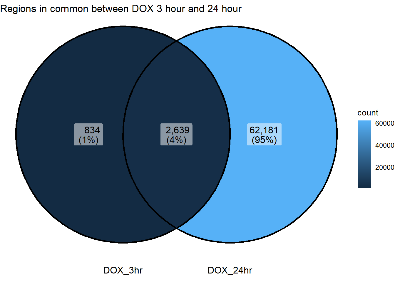

Past versions of "DAR venn-5.png"

Version	Author	Date
30dc0d7	reneeisnowhere	2025-07-21

ggVennDiagram(list("EPi_3hr"=sig_venn_3hr$EPI_3,"EPI_24hr"=sig_venn_24hr$EPI_24))+
   coord_flip()+
  ggtitle("Regions in common between EPI 3 hour and 24 hour")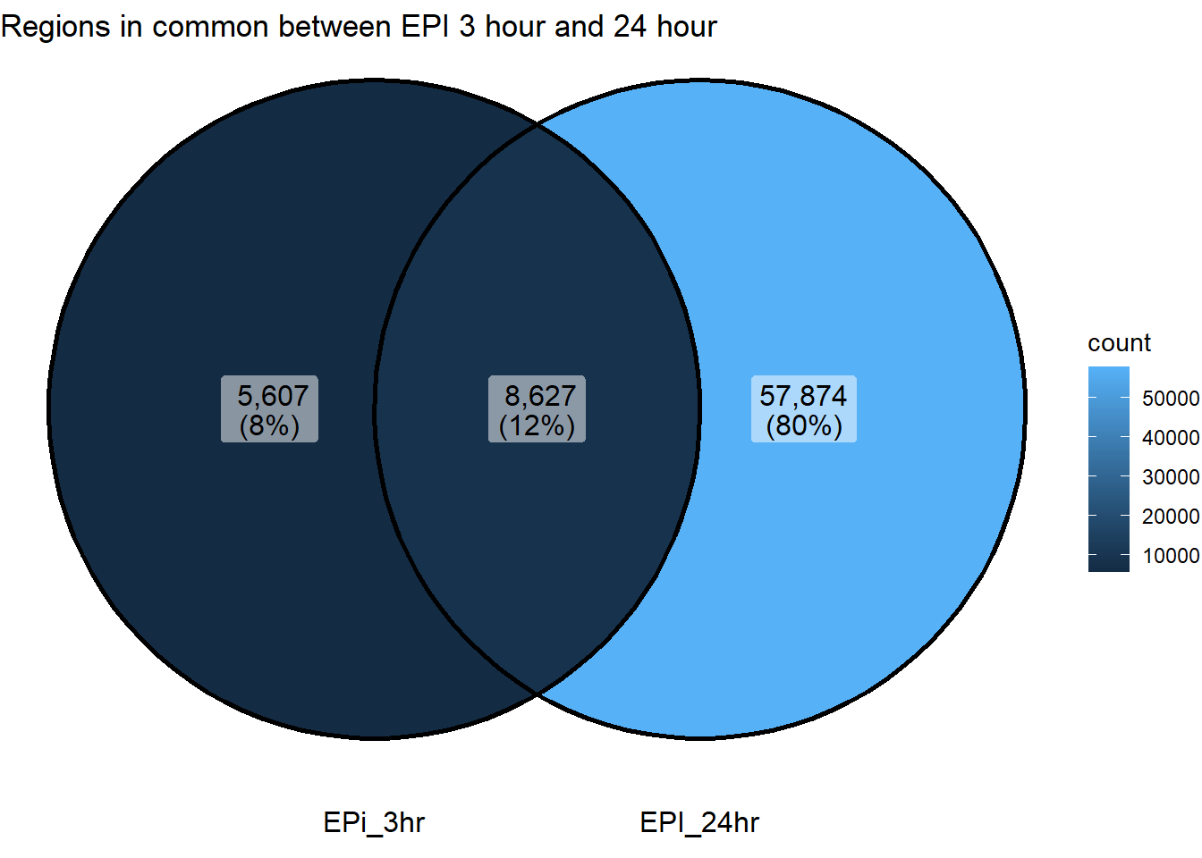

Past versions of "DAR venn-6.png"

Version	Author	Date
30dc0d7	reneeisnowhere	2025-07-21

ggVennDiagram(list("DNR_3hr"=sig_venn_3hr$DNR_3,"DNR_24hr"=sig_venn_24hr$DNR_24))+
   coord_flip()+
  ggtitle("Regions in common between DNR 3 hour and 24 hour")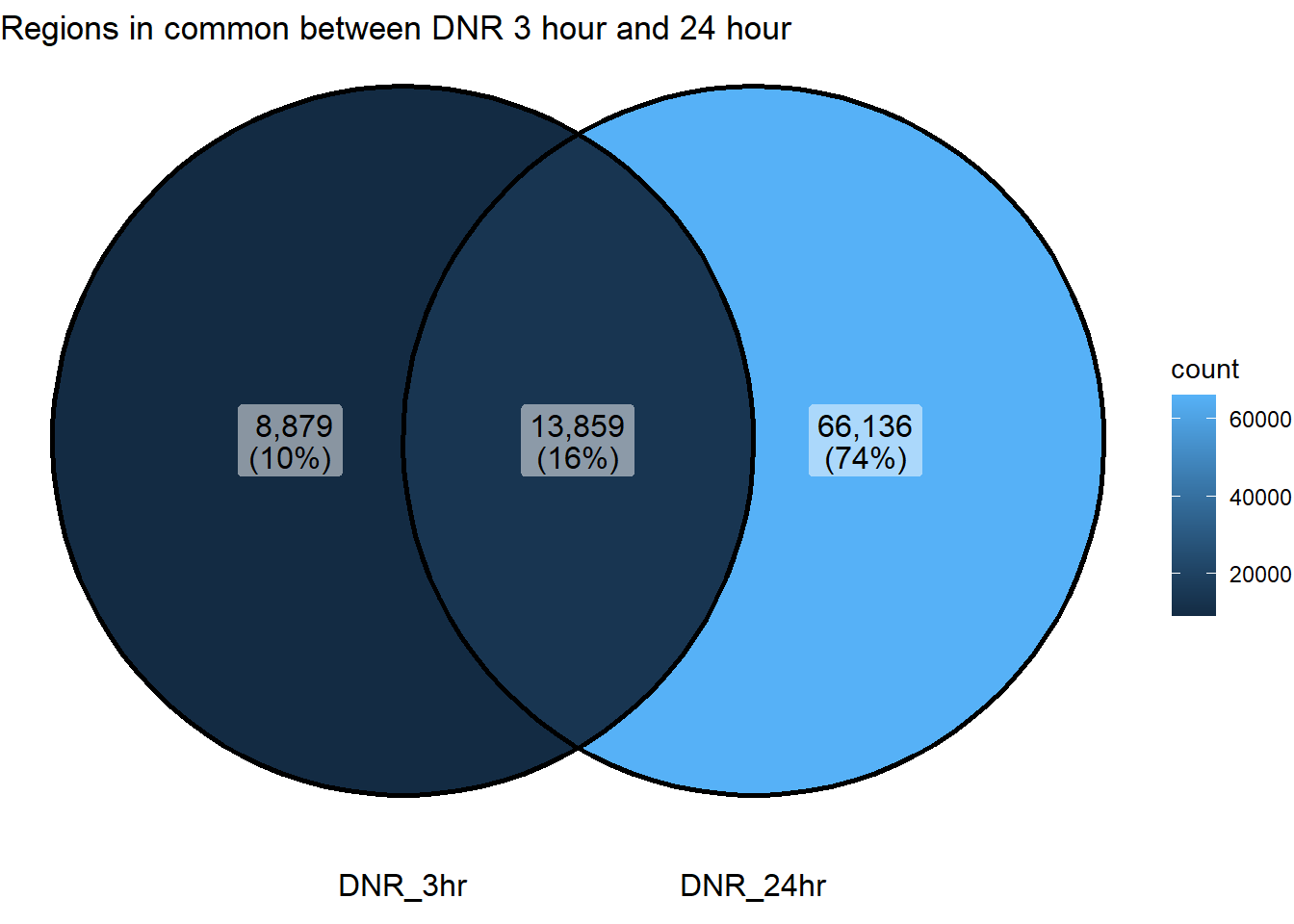

Past versions of "DAR venn-7.png"

Version	Author	Date
30dc0d7	reneeisnowhere	2025-07-21

ggVennDiagram(list("MTX_3hr"=sig_venn_3hr$MTX_3,"MTX_24hr"=sig_venn_24hr$MTX_24))+
   coord_flip()+
  ggtitle("Regions in common between MTX 3 hour and 24 hour")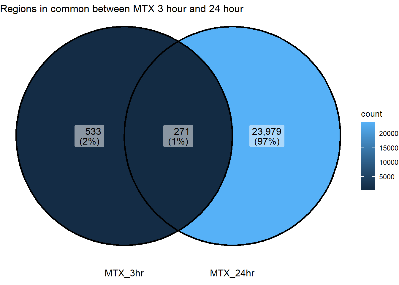

Past versions of "DAR venn-8.png"

Version	Author	Date
30dc0d7	reneeisnowhere	2025-07-21

Proportion of peaks that are DARs

three_hour_df <- all_results %>% 
  dplyr::select(source, genes, logFC,adj.P.Val) %>% 
  mutate(sig_val=if_else(adj.P.Val<0.05,"sig","not_sig")) %>% 
  separate(source, into=c("trt","time"),sep="_") %>% 
  dplyr::filter(time=="3") %>% 
  mutate(trt=factor(trt, levels=c("DOX","EPI","DNR","MTX","TRZ")))

twentyfour_hour_df <- all_results %>% 
  dplyr::select(source, genes, logFC,adj.P.Val) %>% 
  mutate(sig_val=if_else(adj.P.Val<0.05,"sig","not_sig")) %>% 
  separate(source, into=c("trt","time"),sep="_") %>% 
  dplyr::filter(time=="24") %>% 
  mutate(trt=factor(trt, levels=c("DOX","EPI","DNR","MTX","TRZ")))

three_hour_df %>% 
  mutate(sig_val=factor(sig_val,levels = c("not_sig","sig"))) %>% 
  ggplot(., aes(x=trt,fill=sig_val))+
  geom_bar(position="fill")+
  theme_bw()+
  ggtitle("Proportion of significant regions by 3 hours")+
  ylab("proportion")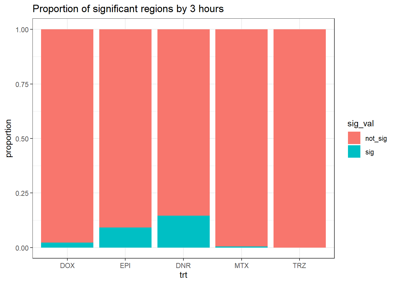

Past versions of "3 and 24 proportion ggplot-1.png"

Version	Author	Date
30dc0d7	reneeisnowhere	2025-07-21

twentyfour_hour_df %>% 
  mutate(sig_val=factor(sig_val,levels = c("not_sig","sig"))) %>% 
  ggplot(., aes(x=trt,fill=sig_val))+
  geom_bar(position="fill")+
  theme_bw()+
  ggtitle("Proportion of significant regions by 24 hours")+
  ylab("proportion")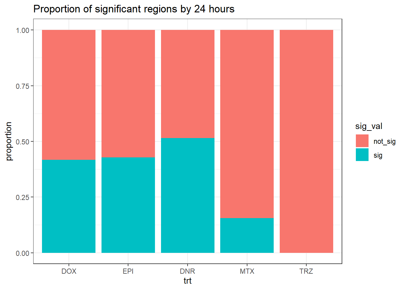

Past versions of "3 and 24 proportion ggplot-2.png"

Version	Author	Date
30dc0d7	reneeisnowhere	2025-07-21

# Ensure consistent trt ordering across both dataframes
ordered_trt <- c("DOX", "EPI", "DNR", "MTX", "TRZ")  # adjust to match your treatment order

# 3-hour plot
plot_3h <- three_hour_df %>%
  mutate(
    sig_val = factor(sig_val, levels = c("not_sig", "sig")),
    trt = factor(trt, levels = ordered_trt)
  ) %>%
  ggplot(aes(x = trt, fill = sig_val)) +
  geom_bar(position = "fill") +
  theme_bw() +
  ggtitle("3 hours") +
  ylab("Proportion") +
  scale_y_continuous(labels = scales::percent)

# 24-hour plot (flipped)
plot_24h <- twentyfour_hour_df %>%
  mutate(
    sig_val = factor(sig_val, levels = c("not_sig", "sig")),
    trt = factor(trt, levels = ordered_trt)
  ) %>%
  ggplot(aes(x = trt, fill = sig_val)) +
  geom_bar(position = "fill") +
  scale_y_reverse(labels = scales::percent) +  # flip it
  theme_bw() +
  ggtitle("24 hours (flipped)") +
  ylab("Proportion")

# Remove x-axis labels from the top plot and y-axis label from the bottom if needed
plot_3h <- plot_3h + theme(axis.title.x = element_blank())
plot_24h <- plot_24h + theme(axis.title.x = element_blank())

# Combine the two using cowplot
combined <- plot_grid(
  plot_3h,
  plot_24h,
  ncol = 1,
  align = "v",
  axis = "lr",  # align left/right axis
  rel_heights = c(1, 1)
)

# Show it
print(combined)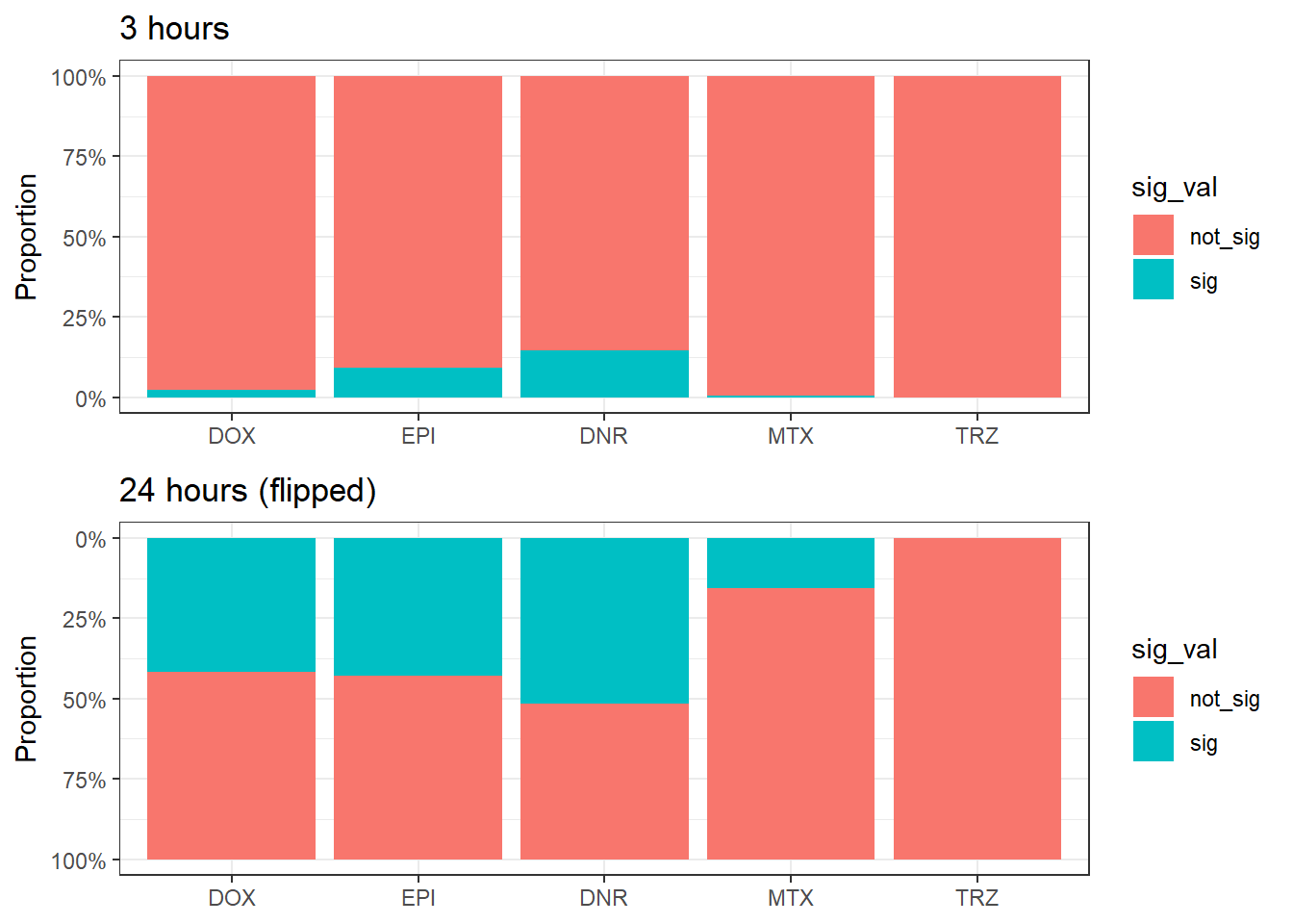

Past versions of unnamed-chunk-4-1.png

Version	Author	Date
30dc0d7	reneeisnowhere	2025-07-21

DOX_sig <- sig_meta_and_loc_split[c("DOX_3", "DOX_24")]

DOXsig_up <- lapply(DOX_sig, function(x) dplyr::filter(x, logFC > 0))
names(DOXsig_up) <- paste0(names(DOXsig_up), "_up")

DOXsig_down <- lapply(DOX_sig, function(x) dplyr::filter(x, logFC < 0))
names(DOXsig_down) <- paste0(names(DOXsig_down), "_down")


DOXsig_up_gr <- lapply(DOXsig_up, function(sub_df) {
  GRanges(
    seqnames = sub_df$seqnames,
    ranges = IRanges(start = sub_df$start, end = sub_df$end),
    mcols = sub_df %>% select(-seqnames, -start, -end)
  )
})

DOXsig_down_gr <- lapply(DOXsig_down, function(sub_df) {
  GRanges(
    seqnames = sub_df$seqnames,
    ranges = IRanges(start = sub_df$start, end = sub_df$end),
    mcols = sub_df %>% select(-seqnames, -start, -end)
  )
})

output_dir <- "data/Final_four_data/re_analysis/motif_beds_centered"

# Create output folder if needed
dir.create(output_dir, showWarnings = FALSE)

# Loop through each BED file
for (name in names(DOXsig_down_gr)) {
  gr <- DOXsig_down_gr[[name]]
  
  # Recenter each region to 200 bp around its midpoint
  gr_centered <- resize(gr, width = 200, fix = "center")
  
  # Export to BED (auto converts to 0-based)
  export(gr_centered, con = file.path(output_dir, paste0(name, "DOXsig_down_centered.bed")), format = "BED")
}

# Loop through each BED file
for (name in names(DOXsig_up_gr)) {
  gr <- DOXsig_up_gr[[name]]
  
  # Recenter each region to 200 bp around its midpoint
  gr_centered <- resize(gr, width = 200, fix = "center")
  
  # Export to BED (auto converts to 0-based)
  export(gr_centered, con = file.path(output_dir, paste0(name, "DOXsig_up_centered.bed")), format = "BED")
}

 filt_DOX24_notup <- all_results %>% 
  dplyr::filter (source=="DOX_24") %>% 
  dplyr::filter(!genes %in% DOXsig_up$DOX_24_up$genes) %>% 
  separate(rowname, into = c("seqnames", "start", "end"), sep = "\\.", convert = TRUE) 

filt_DOX24_notdown <- all_results %>% 
  dplyr::filter (source=="DOX_24") %>% 
  dplyr::filter(!genes %in% DOXsig_down$DOX_24_down$genes) %>% 
  separate(rowname, into = c("seqnames", "start", "end"), sep = "\\.", convert = TRUE) 

# Now convert to GRanges
filt_DOX24_notup_gr <- GRanges(
  seqnames = filt_DOX24_notup$seqnames,
  ranges = IRanges(start = filt_DOX24_notup$start, end = filt_DOX24_notup$end),
  mcols = filt_DOX24_notup %>% select(-seqnames, -start, -end)
)
filt_DOX24_notdown_gr <- GRanges(
  seqnames = filt_DOX24_notdown$seqnames,
  ranges = IRanges(start = filt_DOX24_notdown$start, end = filt_DOX24_notdown$end),
  mcols = filt_DOX24_notdown %>% select(-seqnames, -start, -end)
)
DOX_not_list_gr <- list("DOX24_notup"=filt_DOX24_notup_gr,"DOX24_notdown"=filt_DOX24_notdown_gr)
# for (name in names(DOX_not_list)) {
#   gr <- DOX_not_list[[name]]
#   
#   # Recenter each region to 200 bp around its midpoint
#   gr_centered <- resize(gr, width = 200, fix = "center")
#   
#   # Export to BED (auto converts to 0-based)
#   export(gr_centered, con = file.path(output_dir, paste0(name, "DOX24not_centered.bed")), format = "BED")
# }

txdb <- TxDb.Hsapiens.UCSC.hg38.knownGene
Top2b_peaks <- import(con="data/other_papers/ChIP3_TOP2B_CM_87-1.bed",format = "bed",genome="hg38")

# sig_meta_and_loc_split_gr$TOP2B <- Top2b_peaks
### maybe use annotatePeakInBatch from ChIPpeakAnno
# peakAnnoList_Top2b_DAR <- lapply(all_DAR_regions_gr, annotatePeak, tssRegion =c(-2000,2000), TxDb=txdb)
filt_peakAnnoList_Top2b_DAR <- readRDS("data/Final_four_data/re_analysis/filt_Top2B_DAR_annotated_peaks_chipannno.RDS")
peakAnnoList_DOX_DAR <- readRDS("data/Final_four_data/re_analysis/DOX_DAR_annotated_peaks_chipannno.RDS")
 # saveRDS(peakAnnoList_Top2b_DAR, "data/Final_four_data/re_analysis/Top2B_DAR_annotated_peaks_chipannno.RDS")
# filt_peakAnnoList_Top2b_DAR <- lapply(sig_meta_and_loc_split_gr,annotatePeak, tssRegion =c(-2000,2000), TxDb=txdb)
# saveRDS(filt_peakAnnoList_DOX_DAR, "data/Final_four_data/re_analysis/filt_DOX_DAR_annotated_peaks_chipannno.RDS")
# saveRDS(filt_peakAnnoList_Top2b_DAR, "data/Final_four_data/re_analysis/filt_Top2B_DAR_annotated_peaks_chipannno.RDS")
filt_peakAnnoList_DOX_DAR <- readRDS( "data/Final_four_data/re_analysis/filt_DOX_DAR_annotated_peaks_chipannno.RDS")

plotAnnoBar(peakAnnoList_DOX_DAR)+
  ggtitle ("Genomic Feature Distribution, all DAR no filtering\n should look identical")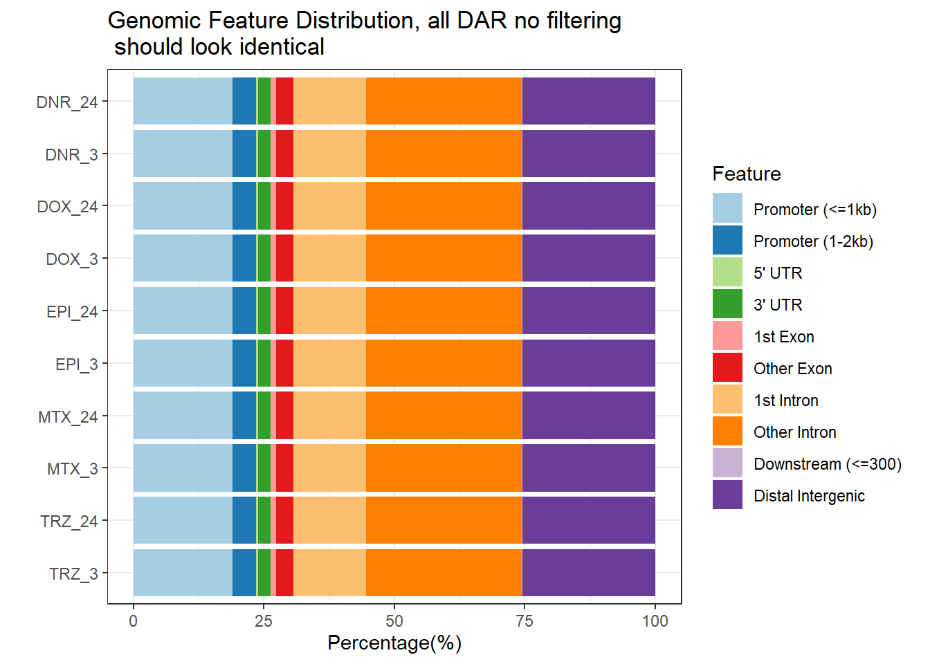

Past versions of "Genomic Features-1.png"

Version	Author	Date
04d6841	reneeisnowhere	2025-06-12

plotAnnoBar(filt_peakAnnoList_DOX_DAR)+
  ggtitle ("Genomic Feature Distribution, Significant regions \n using adj.P.Val <0.05")

Past versions of "Genomic Features-2.png"

Version	Author	Date
04d6841	reneeisnowhere	2025-06-12

plotAnnoBar(filt_peakAnnoList_Top2b_DAR[c(10,4,6,2,8,3,5,1,7)])+
  ggtitle ("Genomic Feature Distribution, Significant regions with Top2B \n using adj.P.Val <0.05")

Past versions of "Genomic Features-3.png"

Version	Author	Date
30dc0d7	reneeisnowhere	2025-07-21

# annotated_peak_TSS_chipanno <-  peakAnnoList_DOX_DAR %>%
#   imap(~ .x %>% tibble::rownames_to_column(var = "rowname") %>%
#          mutate(source = .y)) 

toplistall_RNA <- readRDS("data/other_papers/toplistall_RNA.RDS") %>% 
  mutate(logFC = logFC*(-1))
peakAnnoList_DOX_DAR <- readRDS("data/Final_four_data/re_analysis/DOX_DAR_annotated_peaks_chipannno.RDS")
Assigned_genes_toPeak <- peakAnnoList_DOX_DAR$DOX_24 %>% as.data.frame() %>% 
  dplyr::select(mcols.genes,annotation, geneId, distanceToTSS) %>% 
  dplyr::rename("Peakid"=mcols.genes)


RNA_results <-
toplistall_RNA %>% 
  dplyr::select(time:logFC, adj.P.Val) %>% 
  tidyr::unite("sample",time, id) %>% 
  pivot_wider(., id_cols = c(ENTREZID,SYMBOL),names_from = sample, values_from = c(logFC)) %>% 
  rename_with(~ str_replace(., "hours", "RNA"))


DOX24_degs <- toplistall_RNA %>%
  dplyr::select(time:logFC,adj.P.Val) %>% 
  dplyr::filter(id=="DOX") %>% 
  tidyr::unite("sample",time, id) %>% 
  dplyr::select(sample:SYMBOL,adj.P.Val) %>% 
  dplyr::filter(adj.P.Val<0.05) %>% 
  dplyr::filter(sample=="24_hours_DOX")

DOX3_degs <- toplistall_RNA %>%
  dplyr::select(time:logFC,adj.P.Val) %>% 
  dplyr::filter(id=="DOX") %>% 
  tidyr::unite("sample",time, id) %>% 
  dplyr::select(sample:SYMBOL,adj.P.Val) %>% 
  dplyr::filter(adj.P.Val<0.05) %>% 
  dplyr::filter(sample=="3_hours_DOX")

RNA_all_expressed <-toplistall_RNA %>% 
  dplyr::select(time:logFC,adj.P.Val) %>% 
  dplyr::filter(id=="DOX") %>% 
  dplyr::filter(time=="24_hours") %>% 
  tidyr::unite("sample",time, id) %>% 
  dplyr::select(ENTREZID, SYMBOL)  

Peak_gene_RNA_LFC <- Assigned_genes_toPeak %>% 
  left_join(., RNA_results, by =c("geneId"="ENTREZID"))


entrez_ids <- Assigned_genes_toPeak$geneId  


gene_info <- AnnotationDbi::select(
  org.Hs.eg.db,
  keys = entrez_ids,
  columns = c("SYMBOL"),
  keytype = "ENTREZID"
)
gene_info_collapsed <- gene_info %>%
  group_by(ENTREZID) %>%
  summarise(SYMBOL = paste(unique(SYMBOL), collapse = ","), .groups = "drop")


EPI24_degs <- toplistall_RNA %>%
  dplyr::select(time:logFC,adj.P.Val) %>% 
  dplyr::filter(id=="EPI") %>% 
  tidyr::unite("sample",time, id) %>% 
  dplyr::select(sample:SYMBOL,adj.P.Val) %>% 
  dplyr::filter(adj.P.Val<0.05) %>% 
  dplyr::filter(sample=="24_hours_EPI")

EPI3_degs <- toplistall_RNA %>%
  dplyr::select(time:logFC,adj.P.Val) %>% 
  dplyr::filter(id=="EPI") %>% 
  tidyr::unite("sample",time, id) %>% 
  dplyr::select(sample:SYMBOL,adj.P.Val) %>% 
  dplyr::filter(adj.P.Val<0.05) %>% 
  dplyr::filter(sample=="3_hours_EPI")

DNR24_degs <- toplistall_RNA %>%
  dplyr::select(time:logFC,adj.P.Val) %>% 
  dplyr::filter(id=="DNR") %>% 
  tidyr::unite("sample",time, id) %>% 
  dplyr::select(sample:SYMBOL,adj.P.Val) %>% 
  dplyr::filter(adj.P.Val<0.05) %>% 
  dplyr::filter(sample=="24_hours_DNR")

DNR3_degs <- toplistall_RNA %>%
  dplyr::select(time:logFC,adj.P.Val) %>% 
  dplyr::filter(id=="DNR") %>% 
  tidyr::unite("sample",time, id) %>% 
  dplyr::select(sample:SYMBOL,adj.P.Val) %>% 
  dplyr::filter(adj.P.Val<0.05) %>% 
  dplyr::filter(sample=="3_hours_DNR")

MTX24_degs <- toplistall_RNA %>%
  dplyr::select(time:logFC,adj.P.Val) %>% 
  dplyr::filter(id=="MTX") %>% 
  tidyr::unite("sample",time, id) %>% 
  dplyr::select(sample:SYMBOL,adj.P.Val) %>% 
  dplyr::filter(adj.P.Val<0.05) %>% 
  dplyr::filter(sample=="24_hours_MTX")

MTX3_degs <- toplistall_RNA %>%
  dplyr::select(time:logFC,adj.P.Val) %>% 
  dplyr::filter(id=="MTX") %>% 
  tidyr::unite("sample",time, id) %>% 
  dplyr::select(sample:SYMBOL,adj.P.Val) %>% 
  dplyr::filter(adj.P.Val<0.05) %>% 
  dplyr::filter(sample=="3_hours_MTX")

Exploring DARs and expressed genes

3 hour DOX DAR and expressed RNA genes 2kb

Question, are expressed RNA enriched near (2kb) 3 hour sig DARs vs non-sig DARS?

three_hour_df %>% 
  dplyr::filter(trt=="DOX") %>% 
  left_join(., Assigned_genes_toPeak, by=c("genes"="Peakid")) %>% 
  mutate(EXP_RNA=if_else(geneId %in% RNA_all_expressed$ENTREZID,"exp","not_exp")) %>% 
  dplyr::filter(distanceToTSS>-2000 & distanceToTSS<2000) %>% 
   mutate(sig_val = factor(sig_val, levels = c( "sig","not_sig"))) %>% 
  ggplot(., aes(x=sig_val,fill=EXP_RNA))+
  geom_bar(position="fill")+
  theme_bw()+
  ggtitle("Expressed genes with and without DOX DARs within 2kb  at 3 hours ")+
  ylab("proportion")

Past versions of "3hr expressed 2kb-1.png"

Version	Author	Date
7f3442d	reneeisnowhere	2025-06-13

filtered_df_3hr_exp <-
three_hour_df %>% 
  dplyr::filter(trt == "DOX") %>% 
  left_join(., Assigned_genes_toPeak, by=c("genes"="Peakid")) %>% 
  mutate(EXP_RNA=if_else(geneId %in% RNA_all_expressed$ENTREZID,"exp","not_exp")) %>% 
  dplyr::filter(distanceToTSS>-2000 & distanceToTSS<2000) %>% 
   mutate(sig_val = factor(sig_val, levels = c( "sig","not_sig")))



contingency_table_3hr_exp <- table(filtered_df_3hr_exp$EXP_RNA, filtered_df_3hr_exp$sig_val)
contingency_table_3hr_exp

         
            sig not_sig
  exp       722   24173
  not_exp   258   11441

fisher.test(contingency_table_3hr_exp)

    Fisher's Exact Test for Count Data

data:  contingency_table_3hr_exp
p-value = 0.0001141
alternative hypothesis: true odds ratio is not equal to 1
95 percent confidence interval:
 1.145271 1.535497
sample estimates:
odds ratio 
  1.324524 

3 hour DOX DAR and expressed RNA genes 20kb

Question, are expressed RNA enriched near (20kb) 3 hour sig DARs vs non-sig DARS?

three_hour_df %>% 
  dplyr::filter(trt=="DOX") %>% 
  left_join(., Assigned_genes_toPeak, by=c("genes"="Peakid")) %>% 
  mutate(EXP_RNA=if_else(geneId %in% RNA_all_expressed$ENTREZID,"exp","not_exp")) %>% 
  dplyr::filter(distanceToTSS>-20000 & distanceToTSS<20000) %>% 
   mutate(sig_val = factor(sig_val, levels = c( "sig","not_sig"))) %>% 
  ggplot(., aes(x=sig_val,fill=EXP_RNA))+
  geom_bar(position="fill")+
  theme_bw()+
  ggtitle(" DOX DARs with expressed genes at 3 hours within 20kb")+
  ylab("proportion")

Past versions of "3hr expressed 20kb-1.png"

Version	Author	Date
7f3442d	reneeisnowhere	2025-06-13

filtered_df_3hr_exp20kb <-
three_hour_df %>% 
  dplyr::filter(trt == "DOX") %>% 
  left_join(., Assigned_genes_toPeak, by=c("genes"="Peakid")) %>% 
  mutate(EXP_RNA=if_else(geneId %in% RNA_all_expressed$ENTREZID,"exp","not_exp")) %>% 
  dplyr::filter(distanceToTSS>-20000 & distanceToTSS<20000) %>% 
   mutate(sig_val = factor(sig_val, levels = c( "sig","not_sig")))



contingency_table_3hr_exp20kb <- table(filtered_df_3hr_exp20kb$EXP_RNA, filtered_df_3hr_exp20kb$sig_val)
contingency_table_3hr_exp20kb

         
            sig not_sig
  exp      1595   59956
  not_exp   742   34095

fisher.test(contingency_table_3hr_exp20kb)

    Fisher's Exact Test for Count Data

data:  contingency_table_3hr_exp20kb
p-value = 7.026e-06
alternative hypothesis: true odds ratio is not equal to 1
95 percent confidence interval:
 1.118566 1.336834
sample estimates:
odds ratio 
  1.222358 

24 hour DOX DAR and expressed RNA genes 2kb

Question, are expressed RNA enriched near (2kb) 24 hour sig DARs vs non-sig DARS?

twentyfour_hour_df %>% 
  dplyr::filter(trt=="DOX") %>% 
  left_join(., Assigned_genes_toPeak, by=c("genes"="Peakid")) %>% 
  mutate(EXP_RNA=if_else(geneId %in% RNA_all_expressed$ENTREZID,"exp","not_exp")) %>% 
  dplyr::filter(distanceToTSS>-2000 & distanceToTSS<2000) %>% 
   mutate(sig_val = factor(sig_val, levels = c( "sig","not_sig"))) %>% 
  ggplot(., aes(x=sig_val,fill=EXP_RNA))+
  geom_bar(position="fill")+
  theme_bw()+
  ggtitle("Expressed genes with and without DOX DARs within 2kb  at 24 hours ")+
  ylab("proportion")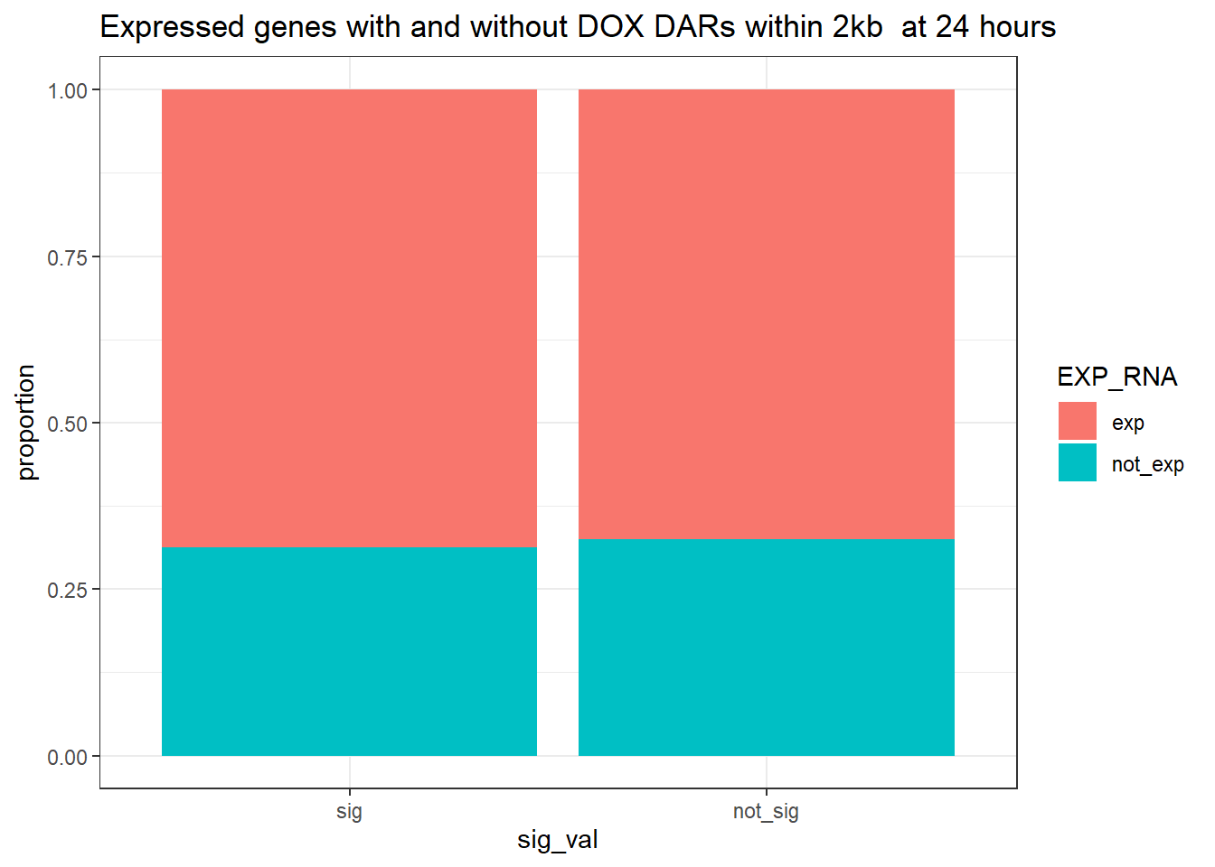

Past versions of "24hr expressed 2kb-1.png"

Version	Author	Date
b377769	reneeisnowhere	2025-06-16
7f3442d	reneeisnowhere	2025-06-13

filtered_df_24hr_exp <-
twentyfour_hour_df %>% 
  dplyr::filter(trt == "DOX") %>% 
  left_join(., Assigned_genes_toPeak, by=c("genes"="Peakid")) %>% 
  mutate(EXP_RNA=if_else(geneId %in% RNA_all_expressed$ENTREZID,"exp","not_exp")) %>% 
  dplyr::filter(distanceToTSS>-2000 & distanceToTSS<2000) %>% 
   mutate(sig_val = factor(sig_val, levels = c( "sig","not_sig")))



contingency_table_24hr_exp <- table(filtered_df_24hr_exp$EXP_RNA, filtered_df_24hr_exp$sig_val)
contingency_table_24hr_exp

         
            sig not_sig
  exp      9482   15413
  not_exp  4301    7398

fisher.test(contingency_table_24hr_exp)

    Fisher's Exact Test for Count Data

data:  contingency_table_24hr_exp
p-value = 0.01514
alternative hypothesis: true odds ratio is not equal to 1
95 percent confidence interval:
 1.010881 1.107718
sample estimates:
odds ratio 
  1.058195 

24 hour DOX DAR and expressed RNA genes 20kb

Question, are expressed RNA enriched near (20kb) 24 hour sig DARs vs non-sig DARS?

twentyfour_hour_df %>% 
  dplyr::filter(trt=="DOX") %>% 
  left_join(., Assigned_genes_toPeak, by=c("genes"="Peakid")) %>% 
  mutate(EXP_RNA=if_else(geneId %in% RNA_all_expressed$ENTREZID,"exp","not_exp")) %>% 
  dplyr::filter(distanceToTSS>-20000 & distanceToTSS<20000) %>% 
   mutate(sig_val = factor(sig_val, levels = c( "sig","not_sig"))) %>% 
  ggplot(., aes(x=sig_val,fill=EXP_RNA))+
  geom_bar(position="fill")+
  theme_bw()+
  ggtitle(" DOX DARs with expressed genes at 24 hours within 20kb")+
  ylab("proportion")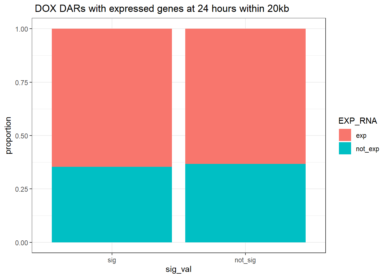

Past versions of "24hr expressed 20kb-1.png"

Version	Author	Date
b377769	reneeisnowhere	2025-06-16
7f3442d	reneeisnowhere	2025-06-13

filtered_df_24hr_exp20kb <-
twentyfour_hour_df %>% 
  dplyr::filter(trt == "DOX") %>% 
  left_join(., Assigned_genes_toPeak, by=c("genes"="Peakid")) %>% 
  mutate(EXP_RNA=if_else(geneId %in% RNA_all_expressed$ENTREZID,"exp","not_exp")) %>% 
  dplyr::filter(distanceToTSS>-20000 & distanceToTSS<20000) %>% 
   mutate(sig_val = factor(sig_val, levels = c( "sig","not_sig")))



contingency_table_24hr_exp20kb <- table(filtered_df_24hr_exp20kb$EXP_RNA, filtered_df_24hr_exp20kb$sig_val)
contingency_table_24hr_exp20kb

         
            sig not_sig
  exp     25562   35989
  not_exp 13965   20872

fisher.test(contingency_table_24hr_exp20kb)

    Fisher's Exact Test for Count Data

data:  contingency_table_24hr_exp20kb
p-value = 1.21e-05
alternative hypothesis: true odds ratio is not equal to 1
95 percent confidence interval:
 1.033450 1.090466
sample estimates:
odds ratio 
    1.0616 

DOX 3 hour DAR and DEGs

Looking at DARs within 2kb of TSS

Question answered below: Are significant DARS within 2kb/20kb of a TSS enriched in DEGs at 3 hours?

three_hour_df %>% 
  dplyr::filter(trt=="DOX") %>% 
  left_join(., Assigned_genes_toPeak, by=c("genes"="Peakid")) %>% 
  mutate(DEG=if_else(geneId %in% DOX3_degs$ENTREZID,"DEG","not_DEG")) %>% 
  dplyr::filter(distanceToTSS>-2000 & distanceToTSS<2000) %>% 
   mutate(sig_val = factor(sig_val, levels = c( "sig","not_sig"))) %>% 
  ggplot(., aes(x=DEG,fill=sig_val))+
  geom_bar(position="fill")+
  theme_bw()+
   ggtitle(" DOX DARs and not-DARs within 2kb of TSS of DEGs at 3 hours")+
  ylab("proportion")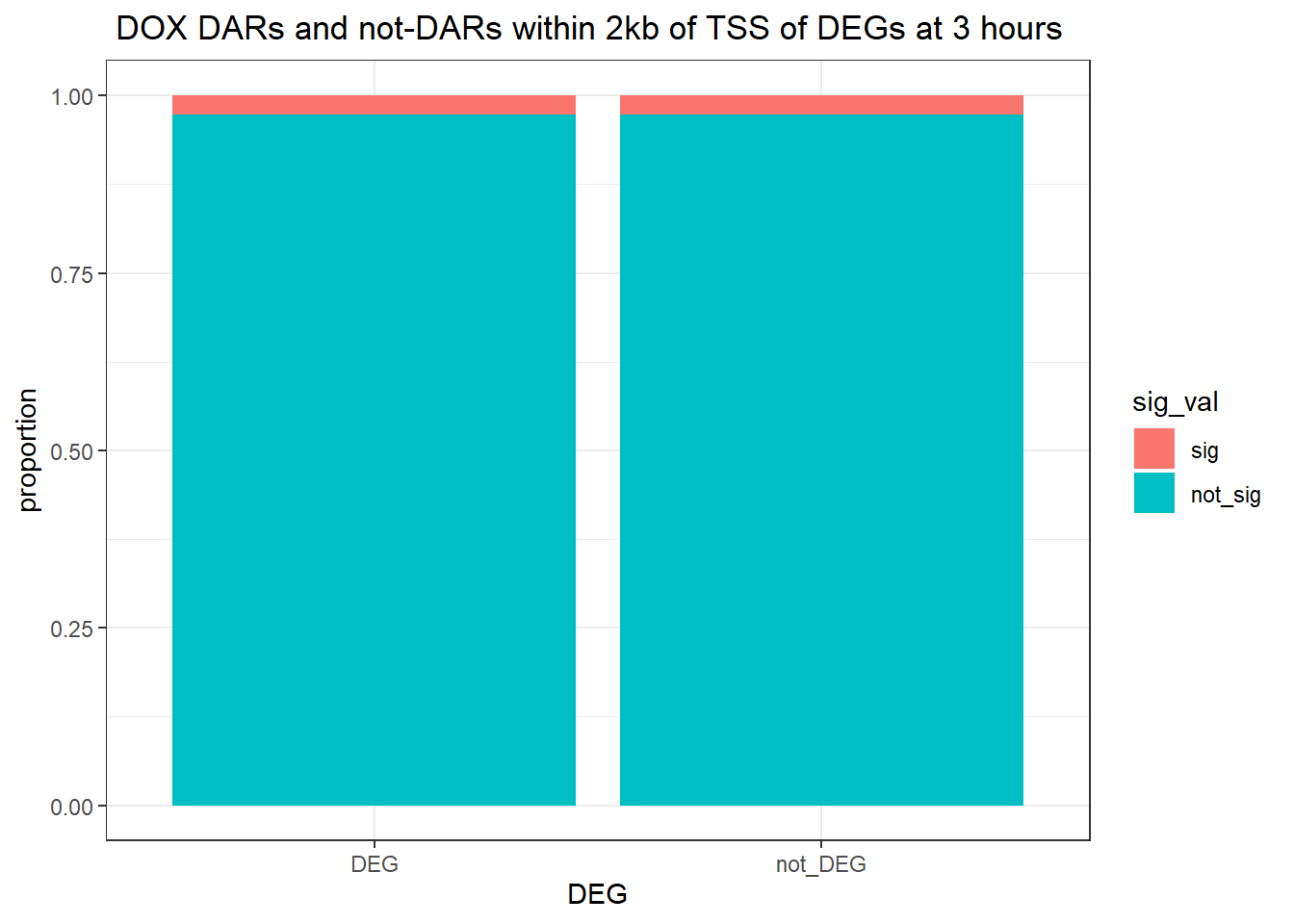

Past versions of "DOX 2kb 3hr DEGnDAR-1.png"

Version	Author	Date
30dc0d7	reneeisnowhere	2025-07-21

filtered_df_3hr_DOX <-
three_hour_df %>% 
  dplyr::filter(trt == "DOX") %>% 
  left_join(Assigned_genes_toPeak, by = c("genes" = "Peakid")) %>% 
  mutate(DEG = if_else(geneId %in% DOX3_degs$ENTREZID, "DEG", "not_DEG")) %>% 
  dplyr::filter(distanceToTSS> -2000 & distanceToTSS < 2000) %>% 
   mutate(sig_val = factor(sig_val, levels = c( "sig","not_sig")))



contingency_table_3hr_DOX <- table(filtered_df_3hr_DOX$DEG, filtered_df_3hr_DOX$sig_val)
contingency_table_3hr_DOX

         
            sig not_sig
  DEG         1      36
  not_DEG   979   35578

fisher.test(contingency_table_3hr_DOX)

    Fisher's Exact Test for Count Data

data:  contingency_table_3hr_DOX
p-value = 1
alternative hypothesis: true odds ratio is not equal to 1
95 percent confidence interval:
 0.02485041 6.00813519
sample estimates:
odds ratio 
  1.009478 

Looking at DARs within 20kb of TSS

three_hour_df %>% 
  dplyr::filter(trt=="DOX") %>% 
  left_join(., Assigned_genes_toPeak, by=c("genes"="Peakid")) %>% 
  mutate(DEG=if_else(geneId %in% DOX3_degs$ENTREZID,"DEG","not_DEG")) %>% 
  dplyr::filter(distanceToTSS>-20000 & distanceToTSS<20000) %>% 
   mutate(sig_val = factor(sig_val, levels = c( "sig","not_sig"))) %>% 
 ggplot(., aes(x=DEG,fill=sig_val))+
  geom_bar(position="fill")+
  theme_bw()+
  ggtitle(" DOX DARs and not-DARs within 20kb of TSS of DEGs at 3 hours")+
  ylab("proportion")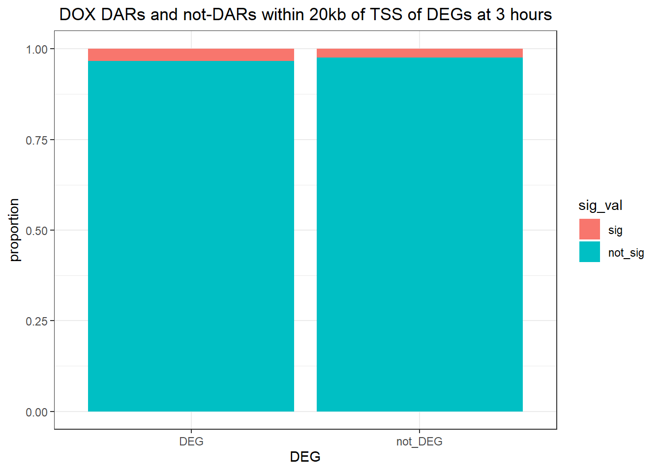

Past versions of "DOX 20kb 3hr DEGnDAR-1.png"

Version	Author	Date
30dc0d7	reneeisnowhere	2025-07-21

filtered_df_3hr20k_DOX <-
three_hour_df %>% 
  dplyr::filter(trt == "DOX") %>% 
  left_join(Assigned_genes_toPeak, by = c("genes" = "Peakid")) %>% 
  mutate(DEG = if_else(geneId %in% DOX3_degs$ENTREZID, "DEG", "not_DEG")) %>% 
  dplyr::filter(distanceToTSS> -20000 & distanceToTSS < 20000) %>% 
   mutate(sig_val = factor(sig_val, levels = c( "sig","not_sig")))



contingency_table_3hr20k_DOX <- table(filtered_df_3hr20k_DOX$DEG, filtered_df_3hr20k_DOX$sig_val)
contingency_table_3hr20k_DOX

         
            sig not_sig
  DEG         4     115
  not_DEG  2333   93936

fisher.test(contingency_table_3hr20k_DOX)

    Fisher's Exact Test for Count Data

data:  contingency_table_3hr20k_DOX
p-value = 0.5398
alternative hypothesis: true odds ratio is not equal to 1
95 percent confidence interval:
 0.3749074 3.6886522
sample estimates:
odds ratio 
  1.400459 

Looking at DARs with all distances to TSS

three_hour_df %>% 
  dplyr::filter(trt=="DOX") %>% 
  left_join(., Assigned_genes_toPeak, by=c("genes"="Peakid")) %>% 
  mutate(DEG=if_else(geneId %in% DOX3_degs$ENTREZID,"DEG","not_DEG")) %>% 
  # dplyr::filter(distanceToTSS>-20000 & distanceToTSS<20000) %>% 
   mutate(sig_val = factor(sig_val, levels = c( "sig","not_sig"))) %>% 

 ggplot(., aes(x=DEG,fill=sig_val))+
  geom_bar(position="fill")+
  theme_bw()+
   ggtitle("DOX DARs and not-DARs within all distance of TSS of DEGs at 3 hours")+
  ylab("proportion")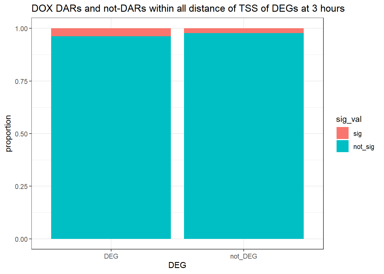

Past versions of "DOX nodist 3hr DEGnDAR-1.png"

Version	Author	Date
30dc0d7	reneeisnowhere	2025-07-21

filtered_df_3hrnodist_DOX <-
three_hour_df %>% 
  dplyr::filter(trt == "DOX") %>% 
  left_join(Assigned_genes_toPeak, by = c("genes" = "Peakid")) %>% 
  mutate(DEG = if_else(geneId %in% DOX3_degs$ENTREZID, "DEG", "not_DEG")) %>% 
  # dplyr::filter(distanceToTSS> -20000 & distanceToTSS < 20000) %>% 
  mutate(sig_val = factor(sig_val, levels = c( "sig","not_sig")))



contingency_table_3hrnodist_DOX <- table(filtered_df_3hrnodist_DOX$DEG, filtered_df_3hrnodist_DOX$sig_val)
contingency_table_3hrnodist_DOX

         
             sig not_sig
  DEG          6     153
  not_DEG   3467  151931

fisher.test(contingency_table_3hrnodist_DOX)

    Fisher's Exact Test for Count Data

data:  contingency_table_3hrnodist_DOX
p-value = 0.1743
alternative hypothesis: true odds ratio is not equal to 1
95 percent confidence interval:
 0.6205303 3.8313098
sample estimates:
odds ratio 
  1.718498 

DOX 24 hour DAR and DEGs

Looking at DARs within 2kb of TSS

Question answered below: Are significant DARS within 2kb/20kb of a TSS enriched in DEGs at 24 hours?

twentyfour_hour_df %>% 
  dplyr::filter(trt=="DOX") %>% 
  left_join(., Assigned_genes_toPeak, by=c("genes"="Peakid")) %>% 
  mutate(DEG=if_else(geneId %in% DOX24_degs$ENTREZID,"DEG","not_DEG")) %>% 
  dplyr::filter(distanceToTSS>-2000 & distanceToTSS<2000) %>% 
   mutate(sig_val = factor(sig_val, levels = c( "sig","not_sig"))) %>% 
 ggplot(., aes(x=DEG,fill=sig_val))+
  geom_bar(position="fill")+
  theme_bw()+
  ggtitle(" DOX DARs and not-DARs within 2kb of TSS of DEGs at 24 hours")+
  ylab("proportion")

Past versions of "DOX 2kb 24hr DEGnDAR-1.png"

Version	Author	Date
30dc0d7	reneeisnowhere	2025-07-21

filtered_df_24hr_DOX <-
twentyfour_hour_df %>% 
  dplyr::filter(trt == "DOX") %>% 
  left_join(Assigned_genes_toPeak, by = c("genes" = "Peakid")) %>% 
  mutate(DEG = if_else(geneId %in% DOX24_degs$ENTREZID, "DEG", "not_DEG")) %>% 
  dplyr::filter(distanceToTSS> -2000 & distanceToTSS < 2000) %>% 
   mutate(sig_val = factor(sig_val, levels = c( "sig","not_sig")))



contingency_table_24hr_DOX <- table(filtered_df_24hr_DOX$DEG, filtered_df_24hr_DOX$sig_val)
contingency_table_24hr_DOX

         
            sig not_sig
  DEG      4810    7211
  not_DEG  8973   15600

fisher.test(contingency_table_24hr_DOX)

    Fisher's Exact Test for Count Data

data:  contingency_table_24hr_DOX
p-value = 9.982e-11
alternative hypothesis: true odds ratio is not equal to 1
95 percent confidence interval:
 1.108569 1.213073
sample estimates:
odds ratio 
  1.159665 

Looking at DARs within 20kb of TSS

twentyfour_hour_df %>% 
  dplyr::filter(trt=="DOX") %>% 
  left_join(., Assigned_genes_toPeak, by=c("genes"="Peakid")) %>% 
  mutate(DEG=if_else(geneId %in% DOX24_degs$ENTREZID,"DEG","not_DEG")) %>% 
  dplyr::filter(distanceToTSS>-20000 & distanceToTSS<20000) %>% 
  mutate(sig_val=factor(sig_val,levels = c("sig","not_sig"))) %>% 
  ggplot(., aes(x=DEG,fill=sig_val))+
  geom_bar(position="fill")+
  theme_bw()+
   ggtitle(" DOX DARs and not-DARs within 20kb of TSS of DEGs at 24 hours")+
  ylab("proportion")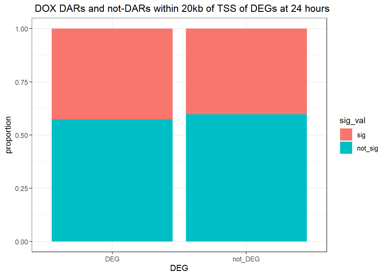

Past versions of "DOX 20kb 24hr DEGnDAR-1.png"

Version	Author	Date
30dc0d7	reneeisnowhere	2025-07-21

filtered_df_24hr20k_DOX <-
twentyfour_hour_df %>% 
  dplyr::filter(trt == "DOX") %>% 
  left_join(Assigned_genes_toPeak, by = c("genes" = "Peakid")) %>% 
  mutate(DEG = if_else(geneId %in% DOX24_degs$ENTREZID, "DEG", "not_DEG")) %>% 
  dplyr::filter(distanceToTSS> -20000 & distanceToTSS < 20000) %>% 
   mutate(sig_val = factor(sig_val, levels = c( "sig","not_sig")))



contingency_table_24hr20k_DOX <- table(filtered_df_24hr20k_DOX$DEG, filtered_df_24hr20k_DOX$sig_val)
contingency_table_24hr20k_DOX

         
            sig not_sig
  DEG     12585   16899
  not_DEG 26942   39962

fisher.test(contingency_table_24hr20k_DOX)

    Fisher's Exact Test for Count Data

data:  contingency_table_24hr20k_DOX
p-value = 2.314e-12
alternative hypothesis: true odds ratio is not equal to 1
95 percent confidence interval:
 1.074263 1.135825
sample estimates:
odds ratio 
  1.104609 

Looking at DARs with all distances to TSS

twentyfour_hour_df %>% 
  dplyr::filter(trt=="DOX") %>% 
  left_join(., Assigned_genes_toPeak, by=c("genes"="Peakid")) %>% 
  mutate(DEG=if_else(geneId %in% DOX24_degs$ENTREZID,"DEG","not_DEG")) %>% 
  # dplyr::filter(distanceToTSS>-20000 & distanceToTSS<20000) %>% 
   mutate(sig_val = factor(sig_val, levels = c( "sig","not_sig"))) %>% 
 ggplot(., aes(x=DEG,fill=sig_val))+
  geom_bar(position="fill")+
  theme_bw()+
  ggtitle(" DOX DARs and not-DARs associated with TSS DEGs at 24 hours")+
  ylab("proportion")

Past versions of "DOX nodist 24hr DEGnDAR-1.png"

Version	Author	Date
30dc0d7	reneeisnowhere	2025-07-21

filtered_df_24hrnodist_DOX <-
twentyfour_hour_df %>% 
  dplyr::filter(trt == "DOX") %>% 
  left_join(Assigned_genes_toPeak, by = c("genes" = "Peakid")) %>% 
  mutate(DEG = if_else(geneId %in% DOX24_degs$ENTREZID, "DEG", "not_DEG")) %>% 
  # dplyr::filter(distanceToTSS> -20000 & distanceToTSS < 20000) %>% 
  mutate(sig_val = factor(sig_val, levels = c( "sig","not_sig")))


contingency_table_24hrnodist_DOX <- table(filtered_df_24hrnodist_DOX$DEG, filtered_df_24hrnodist_DOX$sig_val)
contingency_table_24hrnodist_DOX

         
            sig not_sig
  DEG     18448   24529
  not_DEG 46372   66208

fisher.test(contingency_table_24hrnodist_DOX)

    Fisher's Exact Test for Count Data

data:  contingency_table_24hrnodist_DOX
p-value = 5.671e-10
alternative hypothesis: true odds ratio is not equal to 1
95 percent confidence interval:
 1.049852 1.098289
sample estimates:
odds ratio 
  1.073801 

EPI 3 hour DAR and DEGs

Looking at DARs within 2kb of TSS

three_hour_df %>% 
  dplyr::filter(trt=="EPI") %>% 
  left_join(., Assigned_genes_toPeak, by=c("genes"="Peakid")) %>% 
  mutate(DEG=if_else(geneId %in% EPI3_degs$ENTREZID,"DEG","not_DEG")) %>% 
  dplyr::filter(distanceToTSS>-2000 & distanceToTSS<2000) %>% 
   mutate(sig_val = factor(sig_val, levels = c( "sig","not_sig"))) %>% 
  ggplot(., aes(x=DEG,fill=sig_val))+
  geom_bar(position="fill")+
  theme_bw()+
   ggtitle(" EPI DARs and not-DARs within 2kb of TSS of DEGs at 3 hours")+
  ylab("proportion")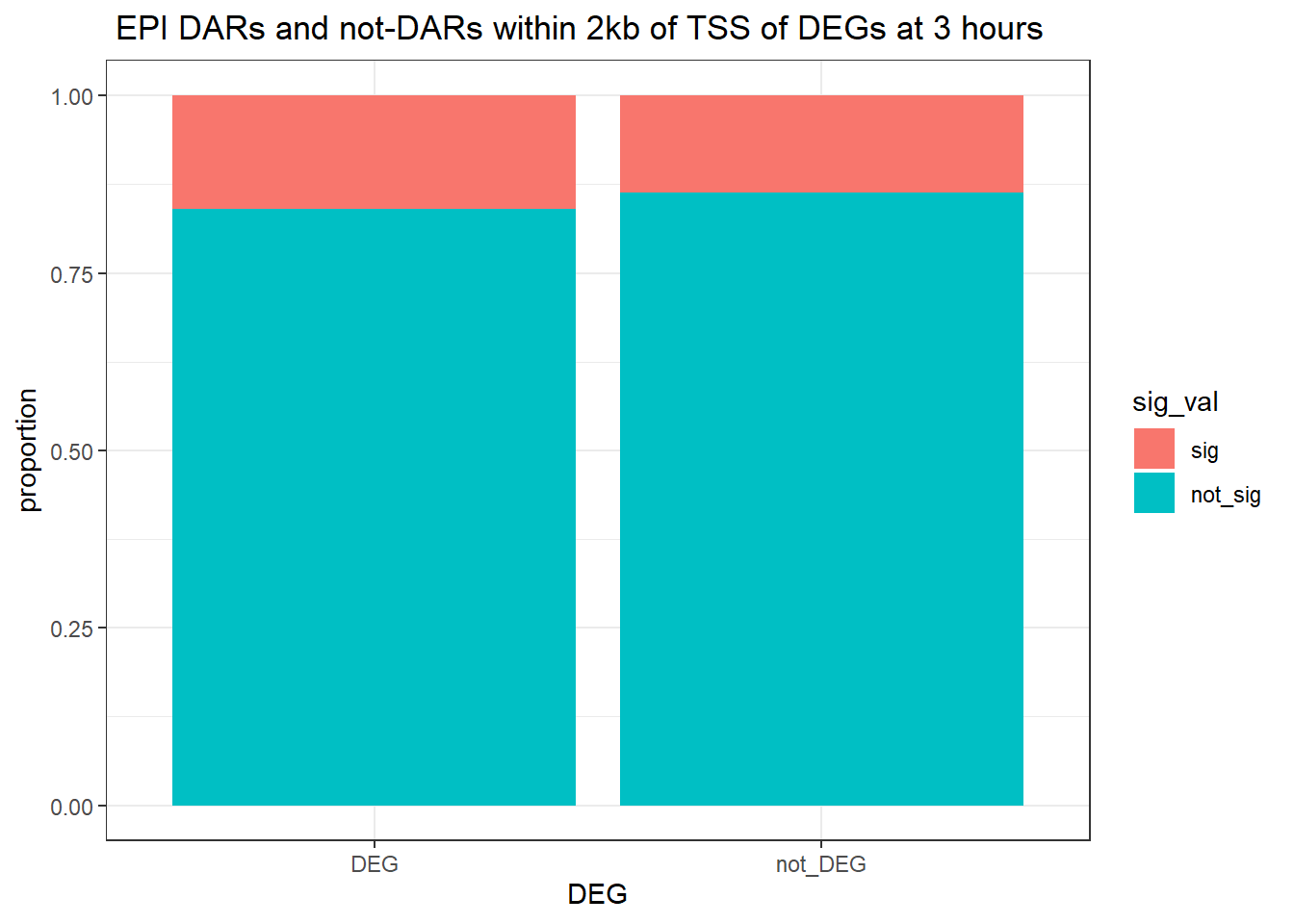

Past versions of "EPI 2kb 3hr DEGnDAR-1.png"

Version	Author	Date
30dc0d7	reneeisnowhere	2025-07-21

filtered_df_3hr_EPI <-
three_hour_df %>% 
  dplyr::filter(trt == "EPI") %>% 
  left_join(Assigned_genes_toPeak, by = c("genes" = "Peakid")) %>% 
  mutate(DEG = if_else(geneId %in% EPI3_degs$ENTREZID, "DEG", "not_DEG")) %>% 
  dplyr::filter(distanceToTSS> -2000 & distanceToTSS < 2000) %>% 
   mutate(sig_val = factor(sig_val, levels = c( "sig","not_sig")))



contingency_table_3hr_EPI <- table(filtered_df_3hr_EPI$DEG, filtered_df_3hr_EPI$sig_val)
contingency_table_3hr_EPI

         
            sig not_sig
  DEG        53     278
  not_DEG  4965   31298

fisher.test(contingency_table_3hr_EPI)

    Fisher's Exact Test for Count Data

data:  contingency_table_3hr_EPI
p-value = 0.2282
alternative hypothesis: true odds ratio is not equal to 1
95 percent confidence interval:
 0.8769852 1.6198073
sample estimates:
odds ratio 
  1.201771 

Looking at DARs within 20kb of TSS

three_hour_df %>% 
  dplyr::filter(trt=="EPI") %>% 
  left_join(., Assigned_genes_toPeak, by=c("genes"="Peakid")) %>% 
  mutate(DEG=if_else(geneId %in% EPI3_degs$ENTREZID,"DEG","not_DEG")) %>% 
  dplyr::filter(distanceToTSS>-20000 & distanceToTSS<20000) %>% 
   mutate(sig_val = factor(sig_val, levels = c( "sig","not_sig"))) %>% 
 ggplot(., aes(x=DEG,fill=sig_val))+
  geom_bar(position="fill")+
  theme_bw()+
  ggtitle(" EPI DARs and not-DARs within 20kb of TSS of DEGs at 3 hours")+
  ylab("proportion")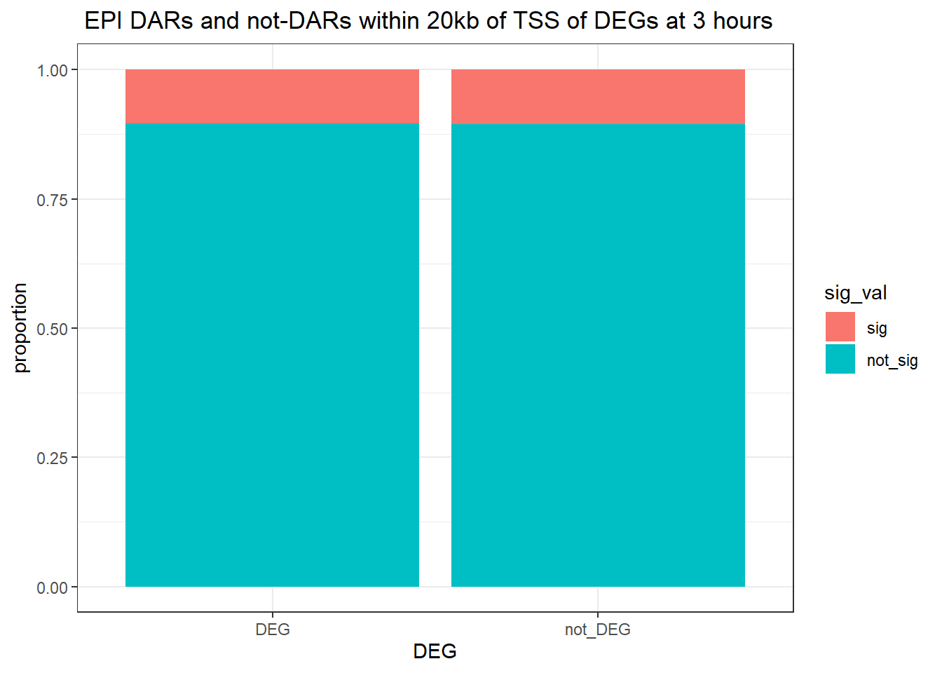

Past versions of "EPI 20kb 3hr DEGnDAR-1.png"

Version	Author	Date
30dc0d7	reneeisnowhere	2025-07-21

filtered_df_3hr20k_EPI <-
three_hour_df %>% 
  dplyr::filter(trt == "EPI") %>% 
  left_join(Assigned_genes_toPeak, by = c("genes" = "Peakid")) %>% 
  mutate(DEG = if_else(geneId %in% EPI3_degs$ENTREZID, "DEG", "not_DEG")) %>% 
  dplyr::filter(distanceToTSS> -20000 & distanceToTSS < 20000) %>% 
   mutate(sig_val = factor(sig_val, levels = c( "sig","not_sig")))



contingency_table_3hr20k_EPI <- table(filtered_df_3hr20k_EPI$DEG, filtered_df_3hr20k_EPI$sig_val)
contingency_table_3hr20k_EPI

         
            sig not_sig
  DEG        98     849
  not_DEG 10020   85421

fisher.test(contingency_table_3hr20k_EPI)

    Fisher's Exact Test for Count Data

data:  contingency_table_3hr20k_EPI
p-value = 0.9152
alternative hypothesis: true odds ratio is not equal to 1
95 percent confidence interval:
 0.7892506 1.2154418
sample estimates:
odds ratio 
 0.9840456 

Looking at DARs with all distances to TSS

three_hour_df %>% 
  dplyr::filter(trt=="EPI") %>% 
  left_join(., Assigned_genes_toPeak, by=c("genes"="Peakid")) %>% 
  mutate(DEG=if_else(geneId %in% EPI3_degs$ENTREZID,"DEG","not_DEG")) %>% 
  # dplyr::filter(distanceToTSS>-20000 & distanceToTSS<20000) %>% 
   mutate(sig_val = factor(sig_val, levels = c( "sig","not_sig"))) %>% 

 ggplot(., aes(x=DEG,fill=sig_val))+
  geom_bar(position="fill")+
  theme_bw()+
   ggtitle("EPI DARs and not-DARs within all distance of TSS of DEGs at 3 hours")+
  ylab("proportion")

Past versions of "EPI nodist 3hr DEGnDAR-1.png"

Version	Author	Date
30dc0d7	reneeisnowhere	2025-07-21

filtered_df_3hrnodist_EPI <-
three_hour_df %>% 
  dplyr::filter(trt == "EPI") %>% 
  left_join(Assigned_genes_toPeak, by = c("genes" = "Peakid")) %>% 
  mutate(DEG = if_else(geneId %in% EPI3_degs$ENTREZID, "DEG", "not_DEG")) %>% 
  # dplyr::filter(distanceToTSS> -20000 & distanceToTSS < 20000) %>% 
  mutate(sig_val = factor(sig_val, levels = c( "sig","not_sig")))



contingency_table_3hrnodist_EPI <- table(filtered_df_3hrnodist_EPI$DEG, filtered_df_3hrnodist_EPI$sig_val)
contingency_table_3hrnodist_EPI

         
             sig not_sig
  DEG        144    1323
  not_DEG  14090  140000

fisher.test(contingency_table_3hrnodist_EPI)

    Fisher's Exact Test for Count Data

data:  contingency_table_3hrnodist_EPI
p-value = 0.3631
alternative hypothesis: true odds ratio is not equal to 1
95 percent confidence interval:
 0.9033813 1.2865204
sample estimates:
odds ratio 
  1.081516 

EPI 24 hour DAR and DEGs

Looking at DARs within 2kb of TSS

twentyfour_hour_df %>% 
  dplyr::filter(trt=="EPI") %>% 
  left_join(., Assigned_genes_toPeak, by=c("genes"="Peakid")) %>% 
  mutate(DEG=if_else(geneId %in% EPI24_degs$ENTREZID,"DEG","not_DEG")) %>% 
  dplyr::filter(distanceToTSS>-2000 & distanceToTSS<2000) %>% 
   mutate(sig_val = factor(sig_val, levels = c( "sig","not_sig"))) %>% 
 ggplot(., aes(x=DEG,fill=sig_val))+
  geom_bar(position="fill")+
  theme_bw()+
  ggtitle(" EPI DARs and not-DARs within 2kb of TSS of DEGs at 24 hours")+
  ylab("proportion")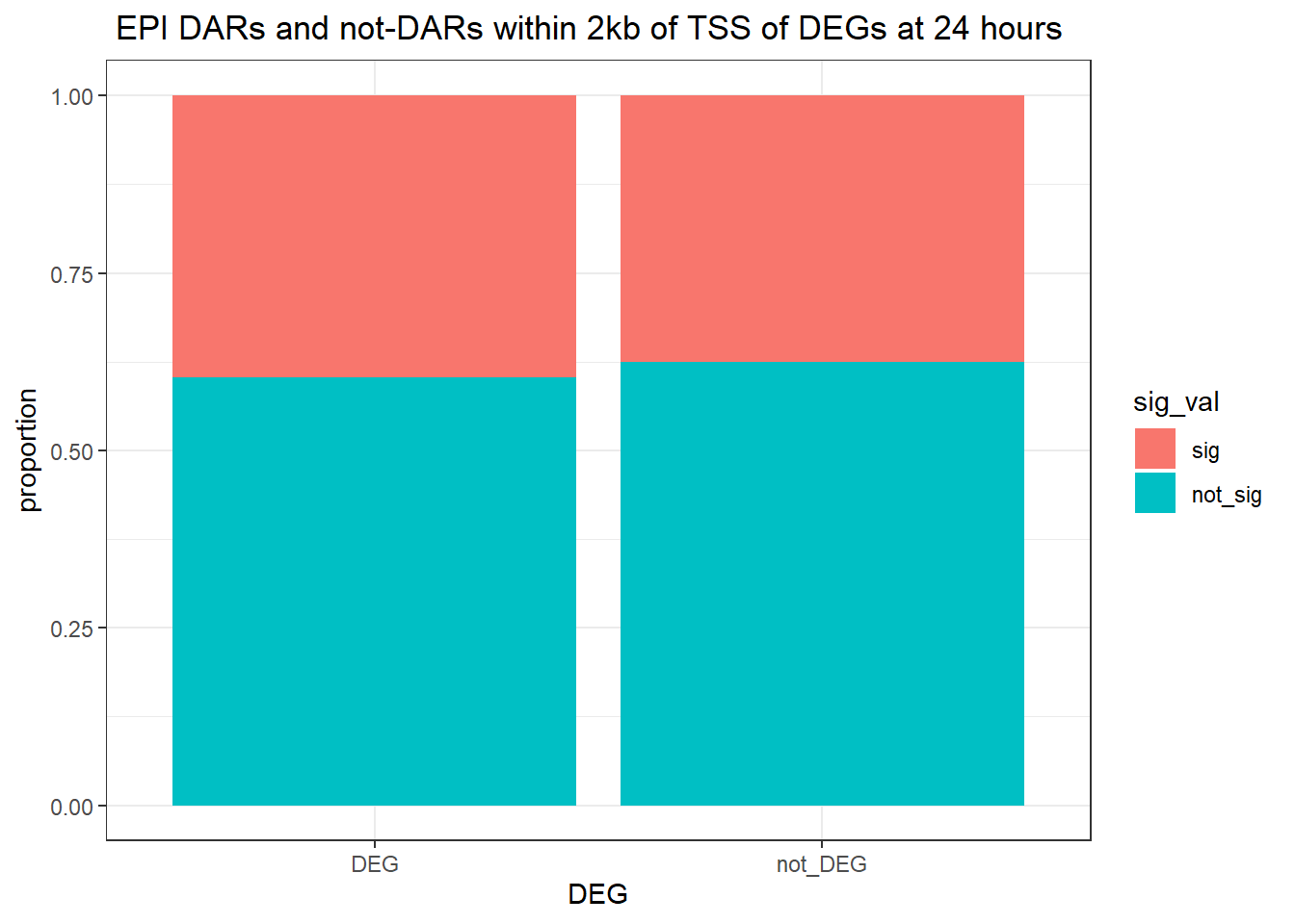

Past versions of "EPI 2kb 24hr DEGnDAR-1.png"

Version	Author	Date
30dc0d7	reneeisnowhere	2025-07-21

filtered_df_24hr_EPI <-
twentyfour_hour_df %>% 
  dplyr::filter(trt == "EPI") %>% 
  left_join(Assigned_genes_toPeak, by = c("genes" = "Peakid")) %>% 
  mutate(DEG = if_else(geneId %in% EPI24_degs$ENTREZID, "DEG", "not_DEG")) %>% 
  dplyr::filter(distanceToTSS> -2000 & distanceToTSS < 2000) %>% 
   mutate(sig_val = factor(sig_val, levels = c( "sig","not_sig")))



contingency_table_24hr_EPI <- table(filtered_df_24hr_EPI$DEG, filtered_df_24hr_EPI$sig_val)
contingency_table_24hr_EPI

         
            sig not_sig
  DEG      4471    6796
  not_DEG  9509   15818

fisher.test(contingency_table_24hr_EPI)

    Fisher's Exact Test for Count Data

data:  contingency_table_24hr_EPI
p-value = 0.0001092
alternative hypothesis: true odds ratio is not equal to 1
95 percent confidence interval:
 1.045388 1.145632
sample estimates:
odds ratio 
  1.094375 

Looking at DARs within 20kb of TSS

twentyfour_hour_df %>% 
  dplyr::filter(trt=="EPI") %>% 
  left_join(., Assigned_genes_toPeak, by=c("genes"="Peakid")) %>% 
  mutate(DEG=if_else(geneId %in% EPI24_degs$ENTREZID,"DEG","not_DEG")) %>% 
  dplyr::filter(distanceToTSS>-20000 & distanceToTSS<20000) %>% 
  mutate(sig_val=factor(sig_val,levels = c("sig","not_sig"))) %>% 
  ggplot(., aes(x=DEG,fill=sig_val))+
  geom_bar(position="fill")+
  theme_bw()+
   ggtitle(" EPI DARs and not-DARs within 20kb of TSS of DEGs at 24 hours")+
  ylab("proportion")

Past versions of "EPI 20kb 24hr DEGnDAR-1.png"

Version	Author	Date
30dc0d7	reneeisnowhere	2025-07-21

filtered_df_24hr20k_EPI <-
twentyfour_hour_df %>% 
  dplyr::filter(trt == "EPI") %>% 
  left_join(Assigned_genes_toPeak, by = c("genes" = "Peakid")) %>% 
  mutate(DEG = if_else(geneId %in% EPI24_degs$ENTREZID, "DEG", "not_DEG")) %>% 
  dplyr::filter(distanceToTSS> -20000 & distanceToTSS < 20000) %>% 
   mutate(sig_val = factor(sig_val, levels = c( "sig","not_sig")))



contingency_table_24hr20k_EPI <- table(filtered_df_24hr20k_EPI$DEG, filtered_df_24hr20k_EPI$sig_val)
contingency_table_24hr20k_EPI

         
            sig not_sig
  DEG     11743   15781
  not_DEG 28707   40157

fisher.test(contingency_table_24hr20k_EPI)

    Fisher's Exact Test for Count Data

data:  contingency_table_24hr20k_EPI
p-value = 0.00553
alternative hypothesis: true odds ratio is not equal to 1
95 percent confidence interval:
 1.011782 1.070907
sample estimates:
odds ratio 
  1.040949 

Looking at DARs with all distances to TSS

twentyfour_hour_df %>% 
  dplyr::filter(trt=="EPI") %>% 
  left_join(., Assigned_genes_toPeak, by=c("genes"="Peakid")) %>% 
  mutate(DEG=if_else(geneId %in% EPI24_degs$ENTREZID,"DEG","not_DEG")) %>% 
  # dplyr::filter(distanceToTSS>-20000 & distanceToTSS<20000) %>% 
   mutate(sig_val = factor(sig_val, levels = c( "sig","not_sig"))) %>% 
 ggplot(., aes(x=DEG,fill=sig_val))+
  geom_bar(position="fill")+
  theme_bw()+
  ggtitle(" EPI DARs and not-DARs associated with TSS DEGs at 24 hours")+
  ylab("proportion")

Past versions of "EPI nodist 24hr DEGnDAR-1.png"

Version	Author	Date
30dc0d7	reneeisnowhere	2025-07-21

filtered_df_24hrnodist_EPI <-
twentyfour_hour_df %>% 
  dplyr::filter(trt == "EPI") %>% 
  left_join(Assigned_genes_toPeak, by = c("genes" = "Peakid")) %>% 
  mutate(DEG = if_else(geneId %in% EPI24_degs$ENTREZID, "DEG", "not_DEG")) %>% 
  # dplyr::filter(distanceToTSS> -20000 & distanceToTSS < 20000) %>% 
  mutate(sig_val = factor(sig_val, levels = c( "sig","not_sig")))


contingency_table_24hrnodist_EPI <- table(filtered_df_24hrnodist_EPI$DEG, filtered_df_24hrnodist_EPI$sig_val)
contingency_table_24hrnodist_EPI

         
            sig not_sig
  DEG     17446   22854
  not_DEG 49055   66202

fisher.test(contingency_table_24hrnodist_EPI)

    Fisher's Exact Test for Count Data

data:  contingency_table_24hrnodist_EPI
p-value = 0.01095
alternative hypothesis: true odds ratio is not equal to 1
95 percent confidence interval:
 1.006782 1.054116
sample estimates:
odds ratio 
  1.030214 

DNR 3 hour DAR and DEGs

Looking at DARs within 2kb of TSS

three_hour_df %>% 
  dplyr::filter(trt=="DNR") %>% 
  left_join(., Assigned_genes_toPeak, by=c("genes"="Peakid")) %>% 
  mutate(DEG=if_else(geneId %in% DNR3_degs$ENTREZID,"DEG","not_DEG")) %>% 
  dplyr::filter(distanceToTSS>-2000 & distanceToTSS<2000) %>% 
   mutate(sig_val = factor(sig_val, levels = c( "sig","not_sig"))) %>% 
  ggplot(., aes(x=DEG,fill=sig_val))+
  geom_bar(position="fill")+
  theme_bw()+
   ggtitle(" DNR DARs and not-DARs within 2kb of TSS of DEGs at 3 hours")+
  ylab("proportion")

Past versions of "DNR 2kb 3hr DEGnDAR-1.png"

Version	Author	Date
30dc0d7	reneeisnowhere	2025-07-21

filtered_df_3hr_DNR <-
three_hour_df %>% 
  dplyr::filter(trt == "DNR") %>% 
  left_join(Assigned_genes_toPeak, by = c("genes" = "Peakid")) %>% 
  mutate(DEG = if_else(geneId %in% DNR3_degs$ENTREZID, "DEG", "not_DEG")) %>% 
  dplyr::filter(distanceToTSS> -2000 & distanceToTSS < 2000) %>% 
   mutate(sig_val = factor(sig_val, levels = c( "sig","not_sig")))



contingency_table_3hr_DNR <- table(filtered_df_3hr_DNR$DEG, filtered_df_3hr_DNR$sig_val)
contingency_table_3hr_DNR

         
            sig not_sig
  DEG       293     616
  not_DEG  8293   27392

fisher.test(contingency_table_3hr_DNR)

    Fisher's Exact Test for Count Data

data:  contingency_table_3hr_DNR
p-value = 1.137e-09
alternative hypothesis: true odds ratio is not equal to 1
95 percent confidence interval:
 1.359397 1.812506
sample estimates:
odds ratio 
   1.57106 

Looking at DARs within 20kb of TSS

three_hour_df %>% 
  dplyr::filter(trt=="DNR") %>% 
  left_join(., Assigned_genes_toPeak, by=c("genes"="Peakid")) %>% 
  mutate(DEG=if_else(geneId %in% DNR3_degs$ENTREZID,"DEG","not_DEG")) %>% 
  dplyr::filter(distanceToTSS>-20000 & distanceToTSS<20000) %>% 
   mutate(sig_val = factor(sig_val, levels = c( "sig","not_sig"))) %>% 
 ggplot(., aes(x=DEG,fill=sig_val))+
  geom_bar(position="fill")+
  theme_bw()+
  ggtitle(" DNR DARs and not-DARs within 20kb of TSS of DEGs at 3 hours")+
  ylab("proportion")

Past versions of "DNR 20kb 3hr DEGnDAR-1.png"

Version	Author	Date
30dc0d7	reneeisnowhere	2025-07-21

filtered_df_3hr20k_DNR <-
three_hour_df %>% 
  dplyr::filter(trt == "DNR") %>% 
  left_join(Assigned_genes_toPeak, by = c("genes" = "Peakid")) %>% 
  mutate(DEG = if_else(geneId %in% DNR3_degs$ENTREZID, "DEG", "not_DEG")) %>% 
  dplyr::filter(distanceToTSS> -20000 & distanceToTSS < 20000) %>% 
   mutate(sig_val = factor(sig_val, levels = c( "sig","not_sig")))



contingency_table_3hr20k_DNR <- table(filtered_df_3hr20k_DNR$DEG, filtered_df_3hr20k_DNR$sig_val)
contingency_table_3hr20k_DNR

         
            sig not_sig
  DEG       488    1936
  not_DEG 15693   78271

fisher.test(contingency_table_3hr20k_DNR)

    Fisher's Exact Test for Count Data

data:  contingency_table_3hr20k_DNR
p-value = 1.345e-05
alternative hypothesis: true odds ratio is not equal to 1
95 percent confidence interval:
 1.134371 1.391268
sample estimates:
odds ratio 
  1.257211 

Looking at DARs with all distances to TSS

three_hour_df %>% 
  dplyr::filter(trt=="DNR") %>% 
  left_join(., Assigned_genes_toPeak, by=c("genes"="Peakid")) %>% 
  mutate(DEG=if_else(geneId %in% DNR3_degs$ENTREZID,"DEG","not_DEG")) %>% 
  # dplyr::filter(distanceToTSS>-20000 & distanceToTSS<20000) %>% 
   mutate(sig_val = factor(sig_val, levels = c( "sig","not_sig"))) %>% 

 ggplot(., aes(x=DEG,fill=sig_val))+
  geom_bar(position="fill")+
  theme_bw()+
   ggtitle("DNR DARs and not-DARs within all distance of TSS of DEGs at 3 hours")+
  ylab("proportion")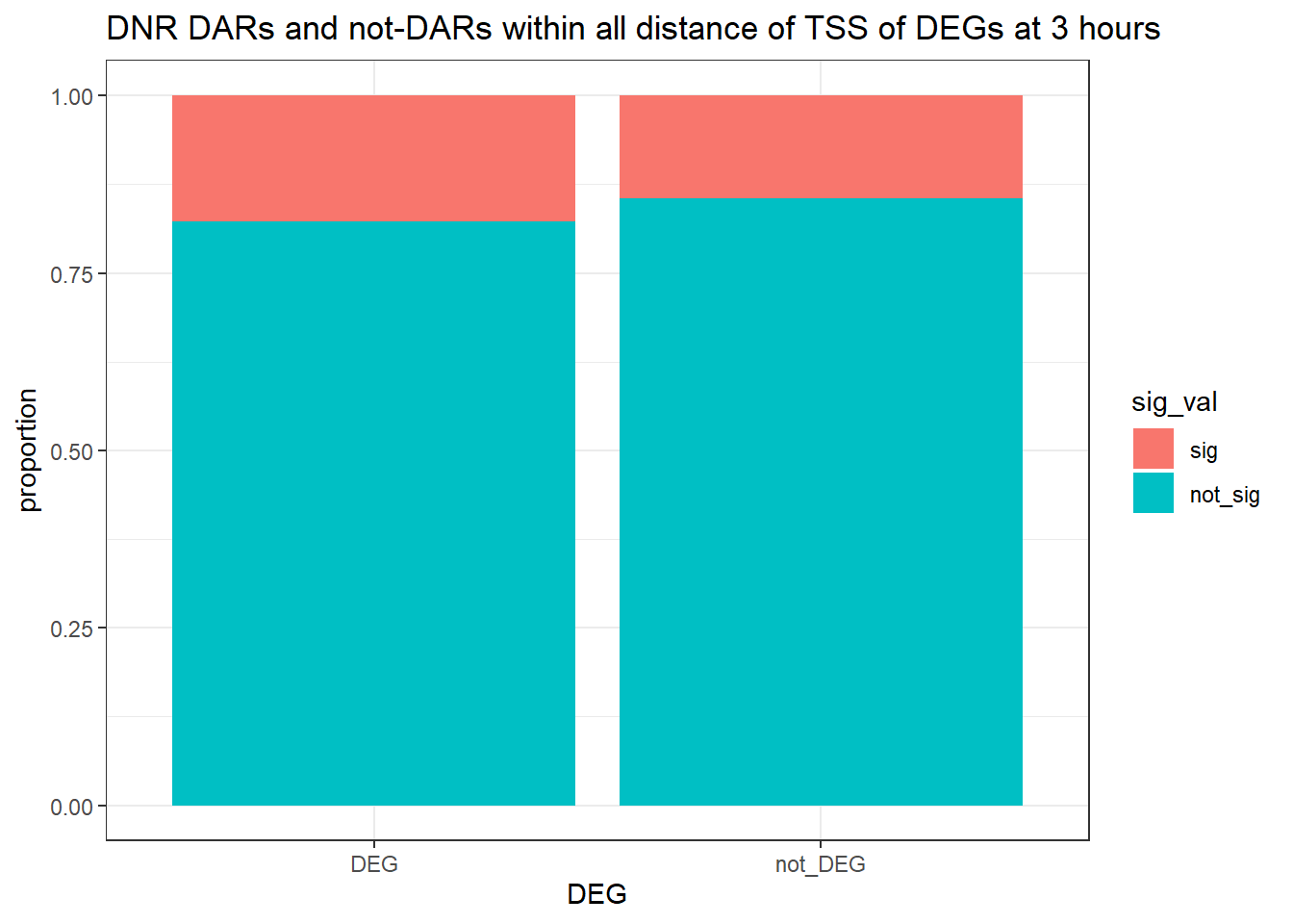

Past versions of "DNR nodist 3hr DEGnDAR-1.png"

Version	Author	Date
30dc0d7	reneeisnowhere	2025-07-21

filtered_df_3hrnodist_DNR <-
three_hour_df %>% 
  dplyr::filter(trt == "DNR") %>% 
  left_join(Assigned_genes_toPeak, by = c("genes" = "Peakid")) %>% 
  mutate(DEG = if_else(geneId %in% DNR3_degs$ENTREZID, "DEG", "not_DEG")) %>% 
  # dplyr::filter(distanceToTSS> -20000 & distanceToTSS < 20000) %>% 
  mutate(sig_val = factor(sig_val, levels = c( "sig","not_sig")))



contingency_table_3hrnodist_DNR <- table(filtered_df_3hrnodist_DNR$DEG, filtered_df_3hrnodist_DNR$sig_val)
contingency_table_3hrnodist_DNR

         
             sig not_sig
  DEG        635    2950
  not_DEG  22103  129869

fisher.test(contingency_table_3hrnodist_DNR)

    Fisher's Exact Test for Count Data

data:  contingency_table_3hrnodist_DNR
p-value = 2.327e-07
alternative hypothesis: true odds ratio is not equal to 1
95 percent confidence interval:
 1.157631 1.380095
sample estimates:
odds ratio 
  1.264751 

DNR 24 hour DAR and DEGs

Looking at DARs within 2kb of TSS

twentyfour_hour_df %>% 
  dplyr::filter(trt=="DNR") %>% 
  left_join(., Assigned_genes_toPeak, by=c("genes"="Peakid")) %>% 
  mutate(DEG=if_else(geneId %in% DNR24_degs$ENTREZID,"DEG","not_DEG")) %>% 
  dplyr::filter(distanceToTSS>-2000 & distanceToTSS<2000) %>% 
   mutate(sig_val = factor(sig_val, levels = c( "sig","not_sig"))) %>% 
 ggplot(., aes(x=DEG,fill=sig_val))+
  geom_bar(position="fill")+
  theme_bw()+
  ggtitle(" DNR DARs and not-DARs within 2kb of TSS of DEGs at 24 hours")+
  ylab("proportion")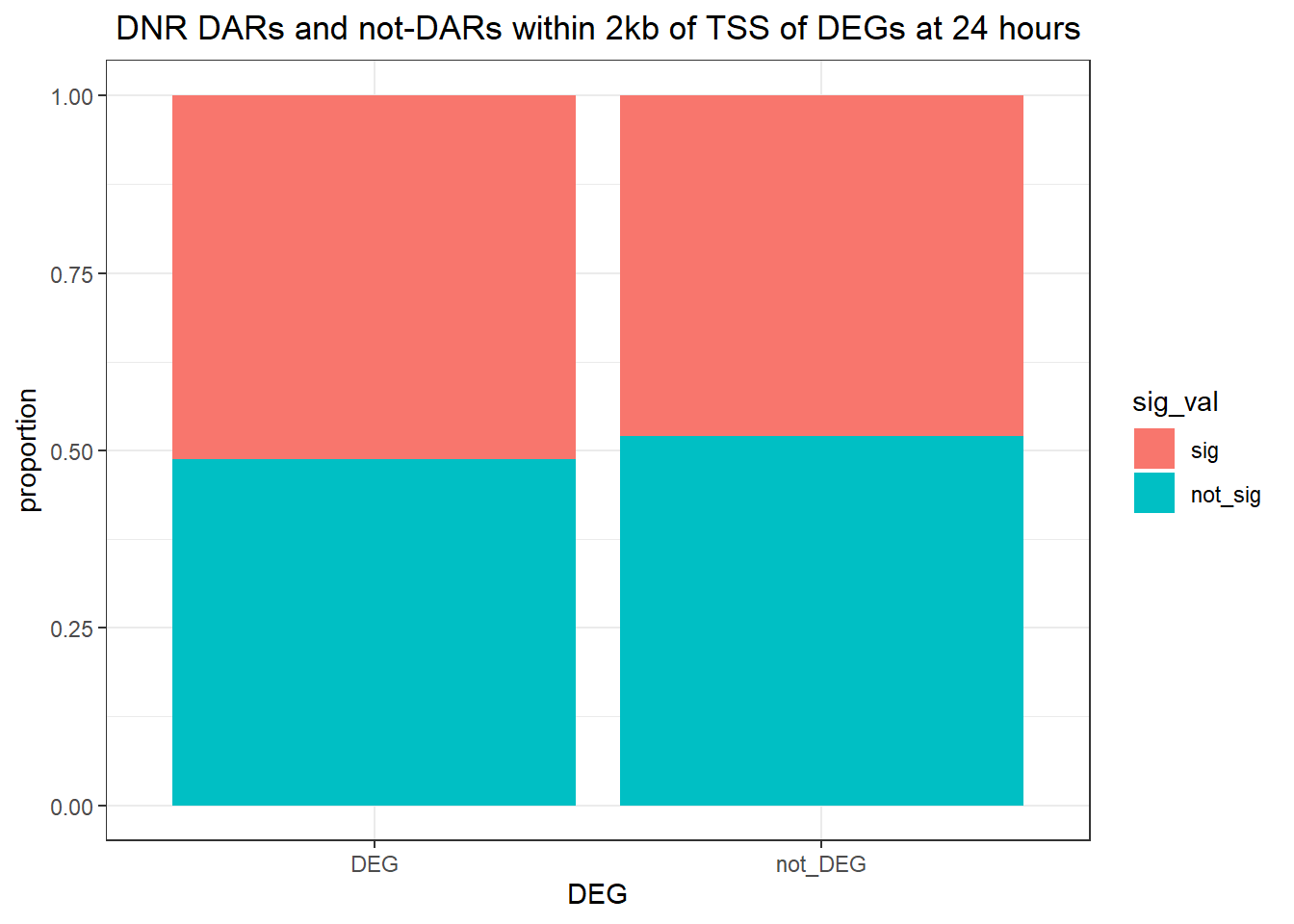

Past versions of "DNR 2kb 24hr DEGnDAR-1.png"

Version	Author	Date
30dc0d7	reneeisnowhere	2025-07-21

filtered_df_24hr_DNR <-
twentyfour_hour_df %>% 
  dplyr::filter(trt == "DNR") %>% 
  left_join(Assigned_genes_toPeak, by = c("genes" = "Peakid")) %>% 
  mutate(DEG = if_else(geneId %in% DNR24_degs$ENTREZID, "DEG", "not_DEG")) %>% 
  dplyr::filter(distanceToTSS> -2000 & distanceToTSS < 2000) %>% 
   mutate(sig_val = factor(sig_val, levels = c( "sig","not_sig")))



contingency_table_24hr_DNR <- table(filtered_df_24hr_DNR$DEG, filtered_df_24hr_DNR$sig_val)
contingency_table_24hr_DNR

         
            sig not_sig
  DEG      6510    6188
  not_DEG 11466   12430

fisher.test(contingency_table_24hr_DNR)

    Fisher's Exact Test for Count Data

data:  contingency_table_24hr_DNR
p-value = 2.291e-09
alternative hypothesis: true odds ratio is not equal to 1
95 percent confidence interval:
 1.092128 1.190967
sample estimates:
odds ratio 
  1.140479 

Looking at DARs within 20kb of TSS

twentyfour_hour_df %>% 
  dplyr::filter(trt=="DNR") %>% 
  left_join(., Assigned_genes_toPeak, by=c("genes"="Peakid")) %>% 
  mutate(DEG=if_else(geneId %in% DNR24_degs$ENTREZID,"DEG","not_DEG")) %>% 
  dplyr::filter(distanceToTSS>-20000 & distanceToTSS<20000) %>% 
  mutate(sig_val=factor(sig_val,levels = c("sig","not_sig"))) %>% 
  ggplot(., aes(x=DEG,fill=sig_val))+
  geom_bar(position="fill")+
  theme_bw()+
   ggtitle(" DNR DARs and not-DARs within 20kb of TSS of DEGs at 24 hours")+
  ylab("proportion")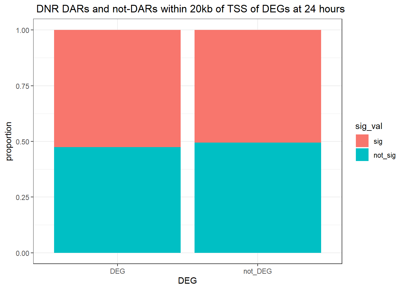

Past versions of "DNR 20kb 24hr DEGnDAR-1.png"

Version	Author	Date
30dc0d7	reneeisnowhere	2025-07-21

filtered_df_24hr20k_DNR <-
twentyfour_hour_df %>% 
  dplyr::filter(trt == "DNR") %>% 
  left_join(Assigned_genes_toPeak, by = c("genes" = "Peakid")) %>% 
  mutate(DEG = if_else(geneId %in% DNR24_degs$ENTREZID, "DEG", "not_DEG")) %>% 
  dplyr::filter(distanceToTSS> -20000 & distanceToTSS < 20000) %>% 
   mutate(sig_val = factor(sig_val, levels = c( "sig","not_sig")))



contingency_table_24hr20k_DNR <- table(filtered_df_24hr20k_DNR$DEG, filtered_df_24hr20k_DNR$sig_val)
contingency_table_24hr20k_DNR

         
            sig not_sig
  DEG     16430   14837
  not_DEG 32946   32175

fisher.test(contingency_table_24hr20k_DNR)

    Fisher's Exact Test for Count Data

data:  contingency_table_24hr20k_DNR
p-value = 1.308e-08
alternative hypothesis: true odds ratio is not equal to 1
95 percent confidence interval:
 1.052518 1.111115
sample estimates:
odds ratio 
  1.081449 

Looking at DARs with all distances to TSS

twentyfour_hour_df %>% 
  dplyr::filter(trt=="DNR") %>% 
  left_join(., Assigned_genes_toPeak, by=c("genes"="Peakid")) %>% 
  mutate(DEG=if_else(geneId %in% DNR24_degs$ENTREZID,"DEG","not_DEG")) %>% 
  # dplyr::filter(distanceToTSS>-20000 & distanceToTSS<20000) %>% 
   mutate(sig_val = factor(sig_val, levels = c( "sig","not_sig"))) %>% 
 ggplot(., aes(x=DEG,fill=sig_val))+
  geom_bar(position="fill")+
  theme_bw()+
  ggtitle(" DNR DARs and not-DARs associated with TSS DEGs at 24 hours")+
  ylab("proportion")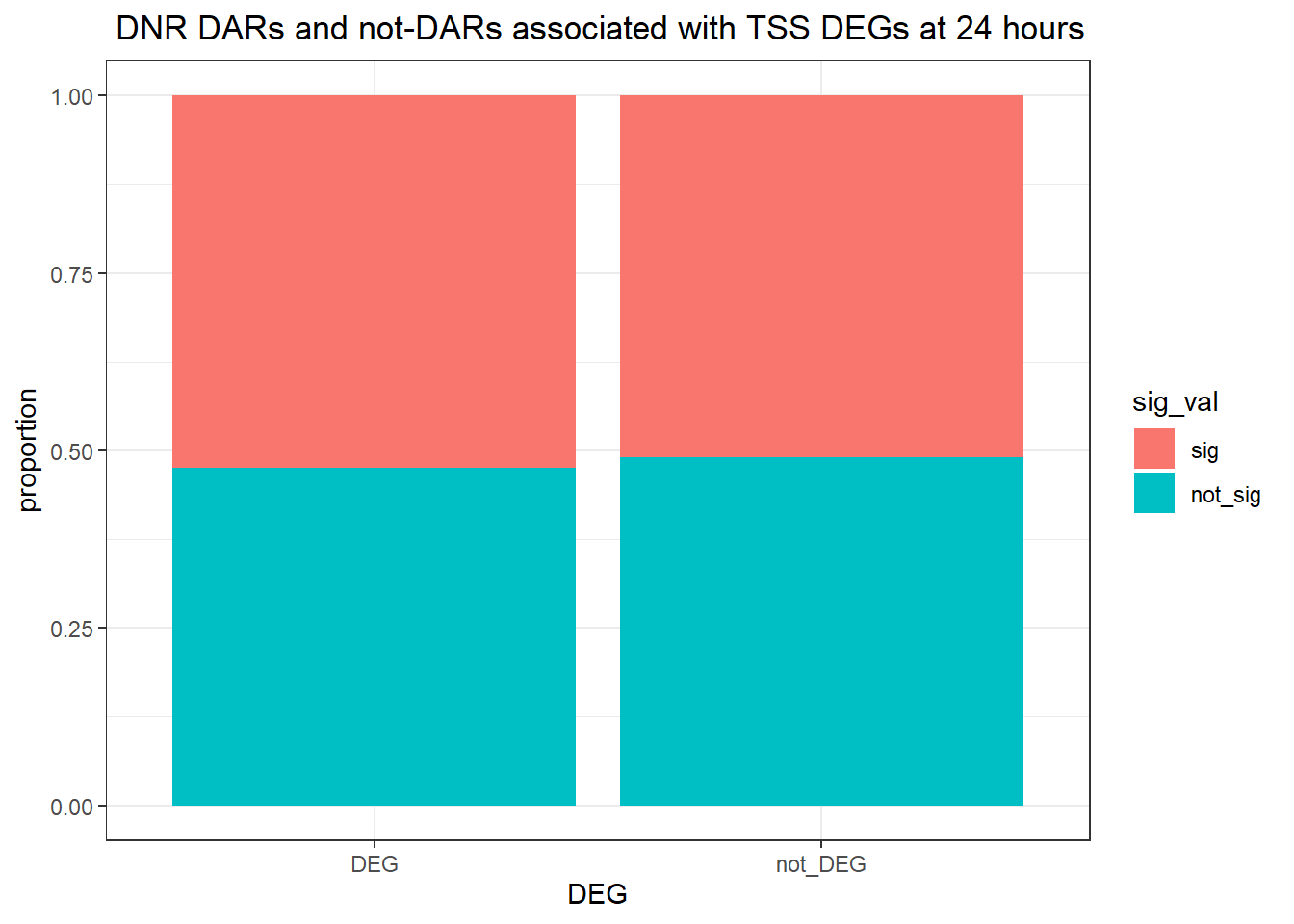

Past versions of "DNR nodist 24hr DEGnDAR-1.png"

Version	Author	Date
30dc0d7	reneeisnowhere	2025-07-21

filtered_df_24hrnodist_DNR <-
twentyfour_hour_df %>% 
  dplyr::filter(trt == "DNR") %>% 
  left_join(Assigned_genes_toPeak, by = c("genes" = "Peakid")) %>% 
  mutate(DEG = if_else(geneId %in% DNR24_degs$ENTREZID, "DEG", "not_DEG")) %>% 
  # dplyr::filter(distanceToTSS> -20000 & distanceToTSS < 20000) %>% 
  mutate(sig_val = factor(sig_val, levels = c( "sig","not_sig")))


contingency_table_24hrnodist_DNR <- table(filtered_df_24hrnodist_DNR$DEG, filtered_df_24hrnodist_DNR$sig_val)
contingency_table_24hrnodist_DNR

         
            sig not_sig
  DEG     23921   21730
  not_DEG 56074   53832

fisher.test(contingency_table_24hrnodist_DNR)

    Fisher's Exact Test for Count Data

data:  contingency_table_24hrnodist_DNR
p-value = 7.133e-07
alternative hypothesis: true odds ratio is not equal to 1
95 percent confidence interval:
 1.033887 1.080254
sample estimates:
odds ratio 
  1.056846 

MTX 3 hour DAR and DEGs

Looking at DARs within 2kb of TSS

three_hour_df %>% 
  dplyr::filter(trt=="MTX") %>% 
  left_join(., Assigned_genes_toPeak, by=c("genes"="Peakid")) %>% 
  mutate(DEG=if_else(geneId %in% MTX3_degs$ENTREZID,"DEG","not_DEG")) %>% 
  dplyr::filter(distanceToTSS>-2000 & distanceToTSS<2000) %>% 
   mutate(sig_val = factor(sig_val, levels = c( "sig","not_sig"))) %>% 
  ggplot(., aes(x=DEG,fill=sig_val))+
  geom_bar(position="fill")+
  theme_bw()+
   ggtitle(" MTX DARs and not-DARs within 2kb of TSS of DEGs at 3 hours")+
  ylab("proportion")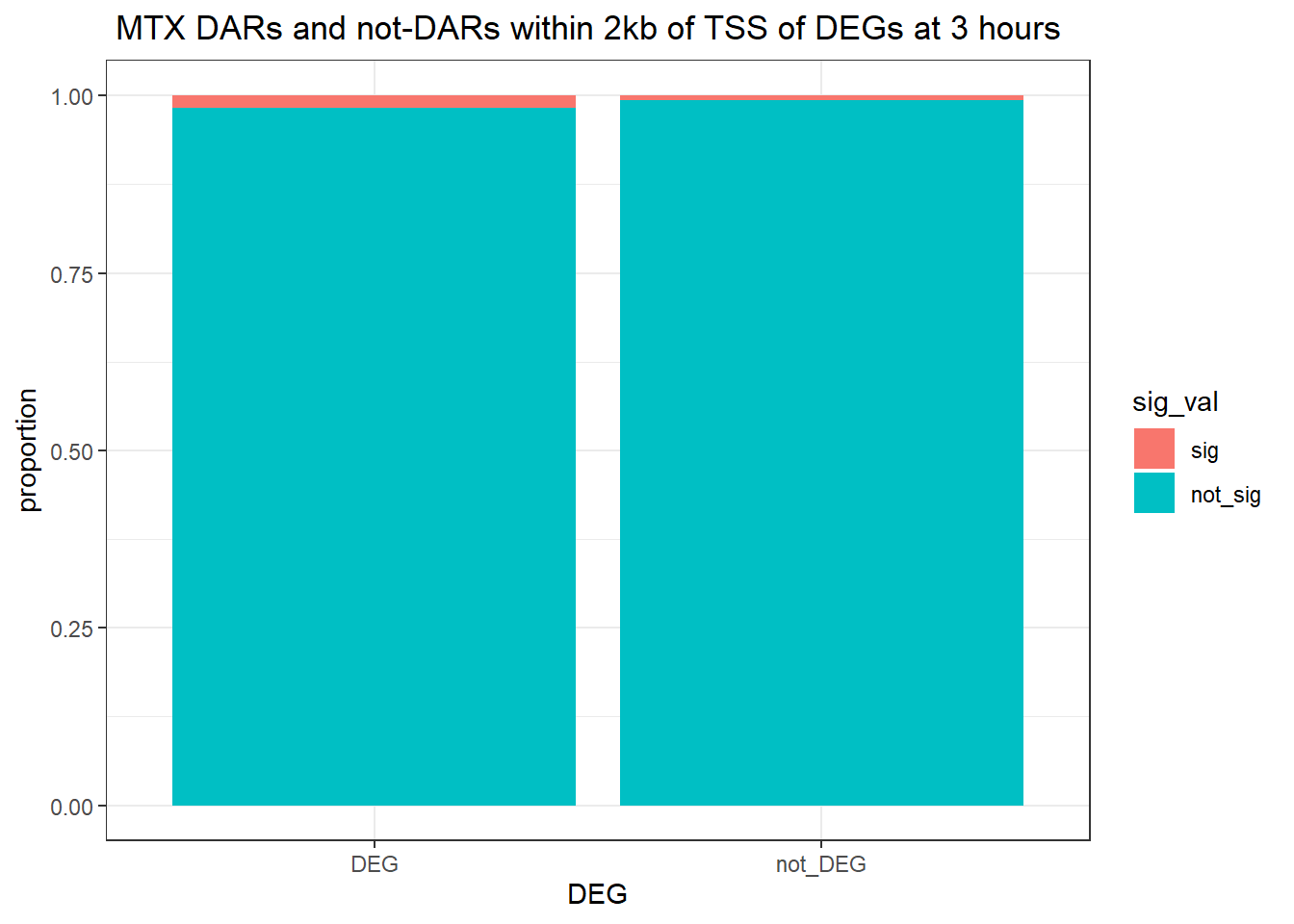

Past versions of "MTX 2kb 3hr DEGnDAR-1.png"

Version	Author	Date
30dc0d7	reneeisnowhere	2025-07-21

filtered_df_3hr_MTX <-
three_hour_df %>% 
  dplyr::filter(trt == "MTX") %>% 
  left_join(Assigned_genes_toPeak, by = c("genes" = "Peakid")) %>% 
  mutate(DEG = if_else(geneId %in% MTX3_degs$ENTREZID, "DEG", "not_DEG")) %>% 
  dplyr::filter(distanceToTSS> -2000 & distanceToTSS < 2000) %>% 
   mutate(sig_val = factor(sig_val, levels = c( "sig","not_sig")))



contingency_table_3hr_MTX <- table(filtered_df_3hr_MTX$DEG, filtered_df_3hr_MTX$sig_val)
contingency_table_3hr_MTX

         
            sig not_sig
  DEG         3     174
  not_DEG   260   36157

fisher.test(contingency_table_3hr_MTX)

    Fisher's Exact Test for Count Data

data:  contingency_table_3hr_MTX
p-value = 0.1355
alternative hypothesis: true odds ratio is not equal to 1
95 percent confidence interval:
 0.4865325 7.2018646
sample estimates:
odds ratio 
  2.397738 

Looking at DARs within 20kb of TSS

three_hour_df %>% 
  dplyr::filter(trt=="MTX") %>% 
  left_join(., Assigned_genes_toPeak, by=c("genes"="Peakid")) %>% 
  mutate(DEG=if_else(geneId %in% MTX3_degs$ENTREZID,"DEG","not_DEG")) %>% 
  dplyr::filter(distanceToTSS>-20000 & distanceToTSS<20000) %>% 
   mutate(sig_val = factor(sig_val, levels = c( "sig","not_sig"))) %>% 
 ggplot(., aes(x=DEG,fill=sig_val))+
  geom_bar(position="fill")+
  theme_bw()+
  ggtitle(" MTX DARs and not-DARs within 20kb of TSS of DEGs at 3 hours")+
  ylab("proportion")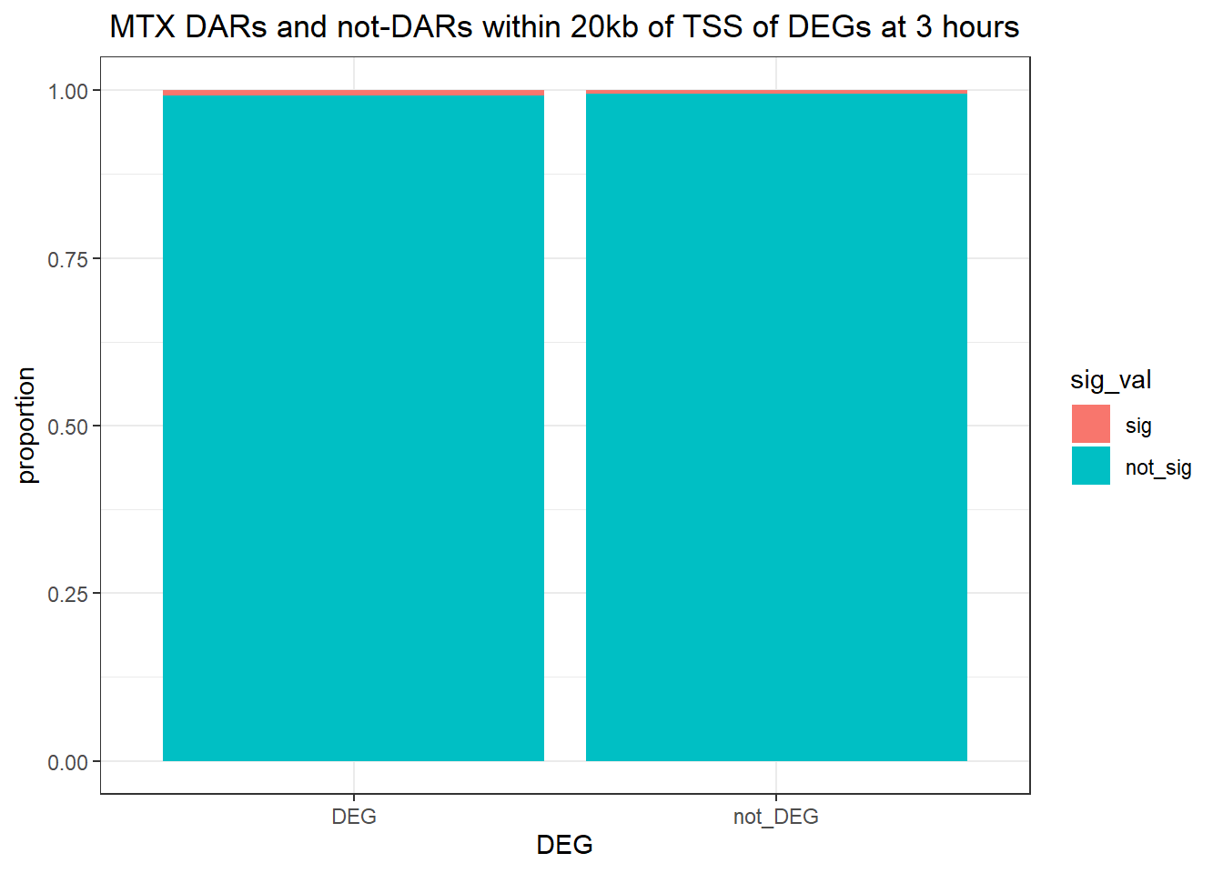

Past versions of "MTX 20kb 3hr DEGnDAR-1.png"

Version	Author	Date
30dc0d7	reneeisnowhere	2025-07-21

filtered_df_3hr20k_MTX <-
three_hour_df %>% 
  dplyr::filter(trt == "MTX") %>% 
  left_join(Assigned_genes_toPeak, by = c("genes" = "Peakid")) %>% 
  mutate(DEG = if_else(geneId %in% MTX3_degs$ENTREZID, "DEG", "not_DEG")) %>% 
  dplyr::filter(distanceToTSS> -20000 & distanceToTSS < 20000) %>% 
   mutate(sig_val = factor(sig_val, levels = c( "sig","not_sig")))



contingency_table_3hr20k_MTX <- table(filtered_df_3hr20k_MTX$DEG, filtered_df_3hr20k_MTX$sig_val)
contingency_table_3hr20k_MTX

         
            sig not_sig
  DEG         4     552
  not_DEG   555   95277

fisher.test(contingency_table_3hr20k_MTX)

    Fisher's Exact Test for Count Data

data:  contingency_table_3hr20k_MTX
p-value = 0.5696
alternative hypothesis: true odds ratio is not equal to 1
95 percent confidence interval:
 0.3365638 3.2211601
sample estimates:
odds ratio 
  1.243982 

Looking at DARs with all distances to TSS

three_hour_df %>% 
  dplyr::filter(trt=="MTX") %>% 
  left_join(., Assigned_genes_toPeak, by=c("genes"="Peakid")) %>% 
  mutate(DEG=if_else(geneId %in% MTX3_degs$ENTREZID,"DEG","not_DEG")) %>% 
  # dplyr::filter(distanceToTSS>-20000 & distanceToTSS<20000) %>% 
   mutate(sig_val = factor(sig_val, levels = c( "sig","not_sig"))) %>% 

 ggplot(., aes(x=DEG,fill=sig_val))+
  geom_bar(position="fill")+
  theme_bw()+
   ggtitle("MTX DARs and not-DARs within all distance of TSS of DEGs at 3 hours")+
  ylab("proportion")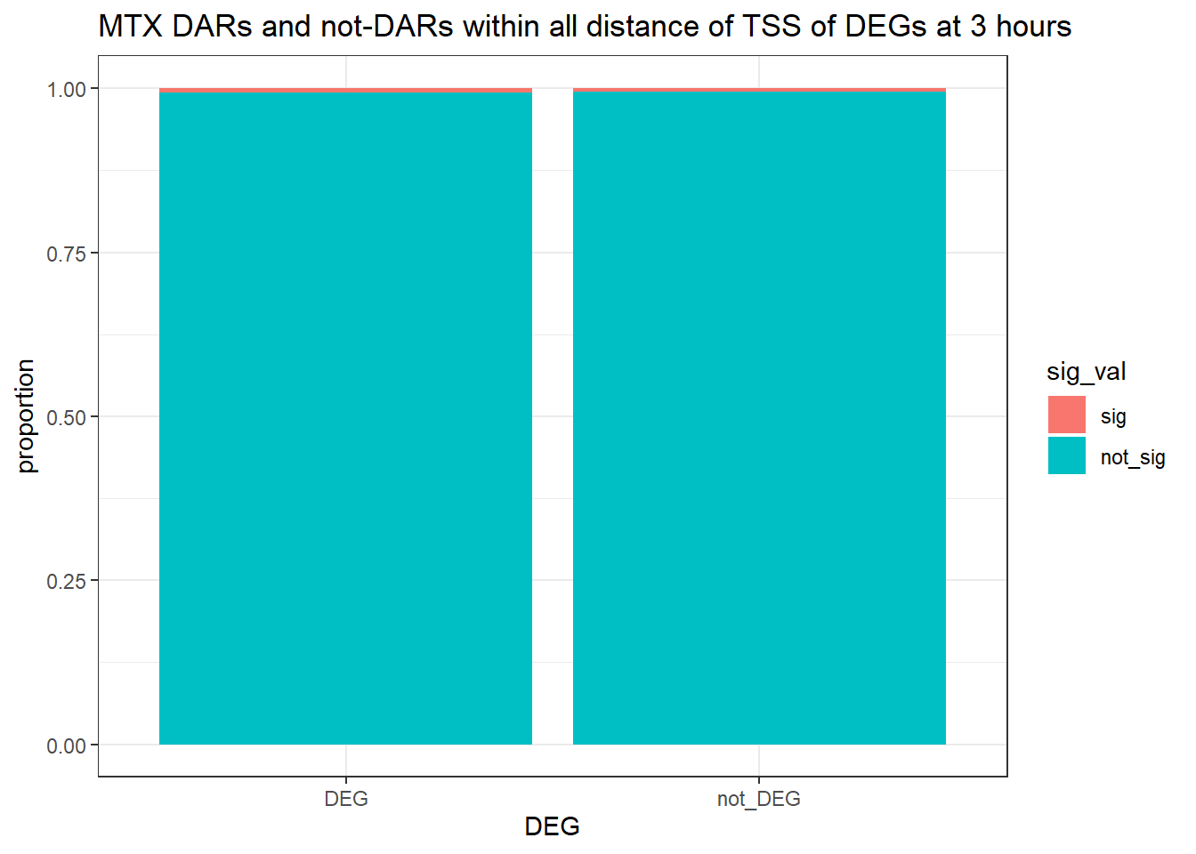

Past versions of "MTX nodist 3hr DEGnDAR-1.png"

Version	Author	Date
30dc0d7	reneeisnowhere	2025-07-21

filtered_df_3hrnodist_MTX <-
three_hour_df %>% 
  dplyr::filter(trt == "MTX") %>% 
  left_join(Assigned_genes_toPeak, by = c("genes" = "Peakid")) %>% 
  mutate(DEG = if_else(geneId %in% MTX3_degs$ENTREZID, "DEG", "not_DEG")) %>% 
  # dplyr::filter(distanceToTSS> -20000 & distanceToTSS < 20000) %>% 
  mutate(sig_val = factor(sig_val, levels = c( "sig","not_sig")))



contingency_table_3hrnodist_MTX <- table(filtered_df_3hrnodist_MTX$DEG, filtered_df_3hrnodist_MTX$sig_val)
contingency_table_3hrnodist_MTX

         
             sig not_sig
  DEG          7     983
  not_DEG    797  153770

fisher.test(contingency_table_3hrnodist_MTX)

    Fisher's Exact Test for Count Data

data:  contingency_table_3hrnodist_MTX
p-value = 0.3681
alternative hypothesis: true odds ratio is not equal to 1
95 percent confidence interval:
 0.5491498 2.8547042
sample estimates:
odds ratio 
  1.373879 

MTX 24 hour DAR and DEGs

Looking at DARs within 2kb of TSS

twentyfour_hour_df %>% 
  dplyr::filter(trt=="MTX") %>% 
  left_join(., Assigned_genes_toPeak, by=c("genes"="Peakid")) %>% 
  mutate(DEG=if_else(geneId %in% MTX24_degs$ENTREZID,"DEG","not_DEG")) %>% 
  dplyr::filter(distanceToTSS>-2000 & distanceToTSS<2000) %>% 
   mutate(sig_val = factor(sig_val, levels = c( "sig","not_sig"))) %>% 
 ggplot(., aes(x=DEG,fill=sig_val))+
  geom_bar(position="fill")+
  theme_bw()+
  ggtitle(" MTX DARs and not-DARs within 2kb of TSS of DEGs at 24 hours")+
  ylab("proportion")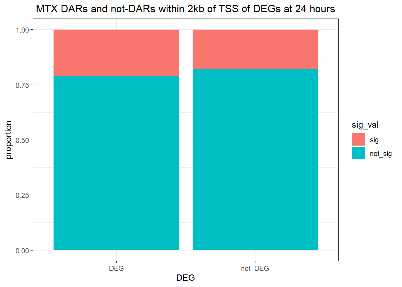

Past versions of "MTX 2kb 24hr DEGnDAR-1.png"

Version	Author	Date
30dc0d7	reneeisnowhere	2025-07-21

filtered_df_24hr_MTX <-
twentyfour_hour_df %>% 
  dplyr::filter(trt == "MTX") %>% 
  left_join(Assigned_genes_toPeak, by = c("genes" = "Peakid")) %>% 
  mutate(DEG = if_else(geneId %in% MTX24_degs$ENTREZID, "DEG", "not_DEG")) %>% 
  dplyr::filter(distanceToTSS> -2000 & distanceToTSS < 2000) %>% 
   mutate(sig_val = factor(sig_val, levels = c( "sig","not_sig")))



contingency_table_24hr_MTX <- table(filtered_df_24hr_MTX$DEG, filtered_df_24hr_MTX$sig_val)
contingency_table_24hr_MTX

         
            sig not_sig
  DEG       451    1695
  not_DEG  6177   28271

fisher.test(contingency_table_24hr_MTX)

    Fisher's Exact Test for Count Data

data:  contingency_table_24hr_MTX
p-value = 0.0004209
alternative hypothesis: true odds ratio is not equal to 1
95 percent confidence interval:
 1.091262 1.356906
sample estimates:
odds ratio 
  1.217777 

Looking at DARs within 20kb of TSS

twentyfour_hour_df %>% 
  dplyr::filter(trt=="MTX") %>% 
  left_join(., Assigned_genes_toPeak, by=c("genes"="Peakid")) %>% 
  mutate(DEG=if_else(geneId %in% MTX24_degs$ENTREZID,"DEG","not_DEG")) %>% 
  dplyr::filter(distanceToTSS>-20000 & distanceToTSS<20000) %>% 
  mutate(sig_val=factor(sig_val,levels = c("sig","not_sig"))) %>% 
  ggplot(., aes(x=DEG,fill=sig_val))+
  geom_bar(position="fill")+
  theme_bw()+
   ggtitle(" MTX DARs and not-DARs within 20kb of TSS of DEGs at 24 hours")+
  ylab("proportion")

Past versions of "MTX 20kb 24hr DEGnDAR-1.png"

Version	Author	Date
30dc0d7	reneeisnowhere	2025-07-21

filtered_df_24hr20k_MTX <-
twentyfour_hour_df %>% 
  dplyr::filter(trt == "MTX") %>% 
  left_join(Assigned_genes_toPeak, by = c("genes" = "Peakid")) %>% 
  mutate(DEG = if_else(geneId %in% MTX24_degs$ENTREZID, "DEG", "not_DEG")) %>% 
  dplyr::filter(distanceToTSS> -20000 & distanceToTSS < 20000) %>% 
   mutate(sig_val = factor(sig_val, levels = c( "sig","not_sig")))



contingency_table_24hr20k_MTX <- table(filtered_df_24hr20k_MTX$DEG, filtered_df_24hr20k_MTX$sig_val)
contingency_table_24hr20k_MTX

         
            sig not_sig
  DEG       982    4474
  not_DEG 14446   76486

fisher.test(contingency_table_24hr20k_MTX)

    Fisher's Exact Test for Count Data

data:  contingency_table_24hr20k_MTX
p-value = 4.718e-05
alternative hypothesis: true odds ratio is not equal to 1
95 percent confidence interval:
 1.081015 1.248390
sample estimates:
odds ratio 
  1.162075 

Looking at DARs with all distances to TSS

twentyfour_hour_df %>% 
  dplyr::filter(trt=="MTX") %>% 
  left_join(., Assigned_genes_toPeak, by=c("genes"="Peakid")) %>% 
  mutate(DEG=if_else(geneId %in% MTX24_degs$ENTREZID,"DEG","not_DEG")) %>% 
  # dplyr::filter(distanceToTSS>-20000 & distanceToTSS<20000) %>% 
   mutate(sig_val = factor(sig_val, levels = c( "sig","not_sig"))) %>% 
 ggplot(., aes(x=DEG,fill=sig_val))+
  geom_bar(position="fill")+
  theme_bw()+
  ggtitle(" MTX DARs and not-DARs associated with TSS DEGs at 24 hours")+
  ylab("proportion")

Past versions of "MTX nodist 24hr DEGnDAR-1.png"

Version	Author	Date
30dc0d7	reneeisnowhere	2025-07-21

twentyfour_hour_df %>% 
  dplyr::filter(trt=="MTX") %>% 
  left_join(., Assigned_genes_toPeak, by=c("genes"="Peakid")) %>% 
  mutate(DEG=if_else(geneId %in% MTX24_degs$ENTREZID,"DEG","not_DEG")) %>% 
  # dplyr::filter(distanceToTSS>-20000 & distanceToTSS<20000) %>% 
   mutate(sig_val = factor(sig_val, levels = c( "sig","not_sig"))) %>% 
 ggplot(., aes(x=sig_val,fill=DEG))+
  geom_bar(position="fill")+
  theme_bw()+
  ggtitle(" FLIPPED !!!")+
  ylab("proportion")

Past versions of "MTX nodist 24hr DEGnDAR-2.png"

Version	Author	Date
30dc0d7	reneeisnowhere	2025-07-21

filtered_df_24hrnodist_MTX <-
twentyfour_hour_df %>% 
  dplyr::filter(trt == "MTX") %>% 
  left_join(Assigned_genes_toPeak, by = c("genes" = "Peakid")) %>% 
  mutate(DEG = if_else(geneId %in% MTX24_degs$ENTREZID, "DEG", "not_DEG")) %>% 
  # dplyr::filter(distanceToTSS> -20000 & distanceToTSS < 20000) %>% 
  mutate(sig_val = factor(sig_val, levels = c( "sig","not_sig")))


contingency_table_24hrnodist_MTX <- table(filtered_df_24hrnodist_MTX$DEG, filtered_df_24hrnodist_MTX$sig_val)
contingency_table_24hrnodist_MTX

         
             sig not_sig
  DEG       1473    6882
  not_DEG  22777  124425

fisher.test(contingency_table_24hrnodist_MTX)

    Fisher's Exact Test for Count Data

data:  contingency_table_24hrnodist_MTX
p-value = 1.885e-07
alternative hypothesis: true odds ratio is not equal to 1
95 percent confidence interval:
 1.102600 1.239305
sample estimates:
odds ratio 
   1.16919 

Contingency matrix and odds ratio for all contrasts

# Question answered below:  Are significant DARS within 2kb/20kb of a TSS enriched in DEGs at 3 hours?

### For each matrix, I want to perform a fisher exact test, and extract the results of that information into a dataframe for graphing.

matrix_names <- c("contingency_table_3hr_DOX",
"contingency_table_3hr20k_DOX",
"contingency_table_24hr_DOX",
"contingency_table_24hr20k_DOX",
"contingency_table_3hr_EPI",
"contingency_table_3hr20k_EPI",
"contingency_table_24hr_EPI",
"contingency_table_24hr20k_EPI",
"contingency_table_3hr_DNR",
"contingency_table_3hr20k_DNR",
"contingency_table_24hr_DNR",
"contingency_table_24hr20k_DNR",
"contingency_table_3hr_MTX",
"contingency_table_3hr20k_MTX",
"contingency_table_24hr_MTX",
"contingency_table_24hr20k_MTX")

results_rowDEG <- data.frame(
  name = character(),
  odds_ratio = numeric(),
  lower_ci = numeric(),
  upper_ci = numeric(),
  p_value = numeric(),
  stringsAsFactors = FALSE
)
for (name in matrix_names) {
  mat <- get(name)  # retrieve matrix by name

  test <- fisher.test(mat)

  results_rowDEG <- rbind(
    results_rowDEG,
    data.frame(
      name = name,
      odds_ratio = unname(test$estimate),
      lower_ci = test$conf.int[1],
      upper_ci = test$conf.int[2],
      p_value = test$p.value
    )
  )
}

plot_results_rowDEG <- results_rowDEG %>% 
  mutate(name= gsub("^contingency_table_","",name)) %>% 
  separate(., name, into=c("time_dist","trt"),sep=("_"), remove = FALSE) %>% 
   extract(time_dist, into = c("time", "distance"), regex = "(\\d+hr)(\\d*k)?", remove = FALSE) %>% 
  mutate(
    distance = ifelse(is.na(distance) | distance == "", "2k", distance)
  ) 

plot_results_rowDEG %>% 
  mutate(time= factor(time, levels =c("3hr","24hr")),
         trt=factor(trt, levels= c("DOX", "EPI", "DNR", "MTX")),
         distance=factor(distance, levels =c("2k","20k"))) %>% 
  # mutate(significant=if_else(p_value <0.05,"TRUE","FALSE")) %>% 
  mutate(
    significant = case_when(
      p_value < 0.001 ~ "***",
      p_value < 0.01 ~ "**",
      p_value < 0.05 ~ "*",
      TRUE ~ ""
    )
  ) %>% 
  ggplot(., aes(x=interaction(trt, distance), y = odds_ratio))+
    geom_point(aes(color = trt), size=4)+
    geom_errorbar(aes(ymin=lower_ci, ymax= upper_ci), width= 0.2)+
   # geom_text(aes(label = significant), vjust = -1.2, color = "black", size = 4) +
  geom_text(
  aes(y = upper_ci + 0.1 * odds_ratio, label = significant),
  hjust = 0,  # aligns text to the left of the y point
  size = 4,
  color = "black"
)+
    geom_hline(yintercept=1, linetype="dashed")+
    theme_classic()+
  facet_wrap(~time, scales = "free_x")+
  coord_flip()+
  ggtitle("Are significant DARs enriched in DEGs?")

Past versions of unnamed-chunk-7-1.png

Version	Author	Date
30dc0d7	reneeisnowhere	2025-07-21

# Question answered below:  Are DEGs  enriched in near significant DARs within 2kb/20kb ?

### For each matrix, I want to perform a fisher exact test, and extract the results of that information into a dataframe for graphing.

matrix_names <- c("contingency_table_3hr_DOX",
"contingency_table_3hr20k_DOX",
"contingency_table_24hr_DOX",
"contingency_table_24hr20k_DOX",
"contingency_table_3hr_EPI",
"contingency_table_3hr20k_EPI",
"contingency_table_24hr_EPI",
"contingency_table_24hr20k_EPI",
"contingency_table_3hr_DNR",
"contingency_table_3hr20k_DNR",
"contingency_table_24hr_DNR",
"contingency_table_24hr20k_DNR",
"contingency_table_3hr_MTX",
"contingency_table_3hr20k_MTX",
"contingency_table_24hr_MTX",
"contingency_table_24hr20k_MTX")

results_rowDAR <- data.frame(
  name = character(),
  odds_ratio = numeric(),
  lower_ci = numeric(),
  upper_ci = numeric(),
  p_value = numeric(),
  stringsAsFactors = FALSE
)
for (name in matrix_names) {
  mat <- get(name)  # retrieve matrix by name
mat_1 <- t(mat)
  test <- fisher.test(mat_1)

  results_rowDAR <- rbind(
    results_rowDAR,
    data.frame(
      name = name,
      odds_ratio = unname(test$estimate),
      lower_ci = test$conf.int[1],
      upper_ci = test$conf.int[2],
      p_value = test$p.value
    )
  )
}

plot_results_rowDAR <- results_rowDAR %>% 
  mutate(name= gsub("^contingency_table_","",name)) %>% 
  separate(., name, into=c("time_dist","trt"),sep=("_"), remove = FALSE) %>% 
   extract(time_dist, into = c("time", "distance"), regex = "(\\d+hr)(\\d*k)?", remove = FALSE) %>% 
  mutate(
    distance = ifelse(is.na(distance) | distance == "", "2k", distance)
  ) 

plot_results_rowDAR %>% 
  mutate(time= factor(time, levels =c("3hr","24hr")),
         trt=factor(trt, levels= c("DOX", "EPI", "DNR", "MTX")),
         distance=factor(distance, levels =c("2k","20k"))) %>% 
  # mutate(significant=if_else(p_value <0.05,"TRUE","FALSE")) %>% 
  mutate(
    significant = case_when(
      p_value < 0.001 ~ "***",
      p_value < 0.01 ~ "**",
      p_value < 0.05 ~ "*",
      TRUE ~ ""
    )
  ) %>% 
  ggplot(., aes(x=interaction(trt, distance), y = odds_ratio))+
    geom_point(aes(color = trt), size=4)+
    geom_errorbar(aes(ymin=lower_ci, ymax= upper_ci), width= 0.2)+
   # geom_text(aes(label = significant), vjust = -1.2, color = "black", size = 4) +
  geom_text(
  aes(y = upper_ci + 0.1 * odds_ratio, label = significant),
  hjust = 0,  # aligns text to the left of the y point
  size = 4,
  color = "black"
)+
    geom_hline(yintercept=1, linetype="dashed")+
    theme_classic()+
  facet_wrap(~time, scales="free_x")+
  coord_flip()+
  ggtitle("Are DEGs enriched near DARs?")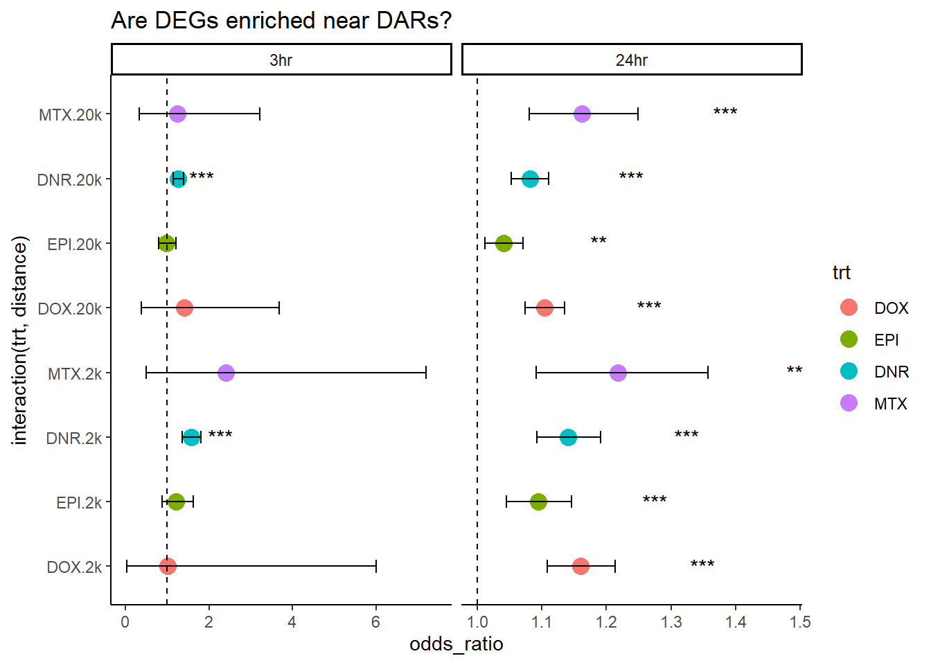

Past versions of unnamed-chunk-9-1.png

Version	Author	Date
30dc0d7	reneeisnowhere	2025-07-21

#   mat_example <- matrix(c(1, 2, 3, 4), nrow = 2, byrow = TRUE,
#               dimnames = list(Group = c("Test", "Reference"),
#                               Outcome = c("Success", "Failure")))
#   mat_example
#   
#   OR= 
# Ref success/Ref failure
# Test success/Test failure
# ​

mat <- contingency_table_3hr_MTX
mat

         
            sig not_sig
  DEG         3     174
  not_DEG   260   36157

fisher.test(mat)

    Fisher's Exact Test for Count Data

data:  mat
p-value = 0.1355
alternative hypothesis: true odds ratio is not equal to 1
95 percent confidence interval:
 0.4865325 7.2018646
sample estimates:
odds ratio 
  2.397738 

tmat <- t(mat)
fisher.test(tmat)

    Fisher's Exact Test for Count Data

data:  tmat
p-value = 0.1355
alternative hypothesis: true odds ratio is not equal to 1
95 percent confidence interval:
 0.4865325 7.2018646
sample estimates:
odds ratio 
  2.397738 

mat <- matrix(c(3, 174, 260, 36157), nrow = 2, byrow = TRUE,
              dimnames = list(c("DEG", "not_DEG"), c("sig", "not_sig")))

# Flip labels, not just orientation
mat_flipped <- matrix(c(3, 260, 174, 36157), nrow = 2, byrow = TRUE,
                      dimnames = list(c("sig", "not_sig"), c("DEG", "not_DEG")))

fisher.test(mat)$estimate        # ~2.4

odds ratio 
  2.397738 

fisher.test(mat_flipped)$estimate  # ~0.417

odds ratio 
  2.397738 

Session information

sessionInfo()

R version 4.4.2 (2024-10-31 ucrt)
Platform: x86_64-w64-mingw32/x64
Running under: Windows 11 x64 (build 26100)

Matrix products: default


locale:
[1] LC_COLLATE=English_United States.utf8 
[2] LC_CTYPE=English_United States.utf8   
[3] LC_MONETARY=English_United States.utf8
[4] LC_NUMERIC=C                          
[5] LC_TIME=English_United States.utf8    

time zone: America/Chicago
tzcode source: internal

attached base packages:
[1] grid      stats4    stats     graphics  grDevices utils     datasets 
[8] methods   base     

other attached packages:
 [1] BSgenome.Hsapiens.UCSC.hg38_1.4.5       
 [2] BSgenome_1.74.0                         
 [3] BiocIO_1.16.0                           
 [4] Biostrings_2.74.1                       
 [5] XVector_0.46.0                          
 [6] ggVennDiagram_1.5.4                     
 [7] data.table_1.17.6                       
 [8] smplot2_0.2.5                           
 [9] cowplot_1.1.3                           
[10] ComplexHeatmap_2.22.0                   
[11] ggrepel_0.9.6                           
[12] plyranges_1.26.0                        
[13] ggsignif_0.6.4                          
[14] eulerr_7.0.2                            
[15] devtools_2.4.5                          
[16] usethis_3.1.0                           
[17] ggpubr_0.6.1                            
[18] BiocParallel_1.40.2                     
[19] scales_1.4.0                            
[20] VennDiagram_1.7.3                       
[21] futile.logger_1.4.3                     
[22] gridExtra_2.3                           
[23] ggfortify_0.4.18                        
[24] edgeR_4.4.2                             
[25] limma_3.62.2                            
[26] rtracklayer_1.66.0                      
[27] org.Hs.eg.db_3.20.0                     
[28] TxDb.Hsapiens.UCSC.hg38.knownGene_3.20.0
[29] GenomicFeatures_1.58.0                  
[30] AnnotationDbi_1.68.0                    
[31] Biobase_2.66.0                          
[32] GenomicRanges_1.58.0                    
[33] GenomeInfoDb_1.42.3                     
[34] IRanges_2.40.1                          
[35] S4Vectors_0.44.0                        
[36] BiocGenerics_0.52.0                     
[37] ChIPseeker_1.42.1                       
[38] RColorBrewer_1.1-3                      
[39] broom_1.0.8                             
[40] kableExtra_1.4.0                        
[41] lubridate_1.9.4                         
[42] forcats_1.0.0                           
[43] stringr_1.5.1                           
[44] dplyr_1.1.4                             
[45] purrr_1.0.4                             
[46] readr_2.1.5                             
[47] tidyr_1.3.1                             
[48] tibble_3.3.0                            
[49] ggplot2_3.5.2                           
[50] tidyverse_2.0.0                         
[51] workflowr_1.7.1                         

loaded via a namespace (and not attached):
  [1] fs_1.6.6                               
  [2] matrixStats_1.5.0                      
  [3] bitops_1.0-9                           
  [4] enrichplot_1.26.6                      
  [5] httr_1.4.7                             
  [6] doParallel_1.0.17                      
  [7] profvis_0.4.0                          
  [8] tools_4.4.2                            
  [9] backports_1.5.0                        
 [10] R6_2.6.1                               
 [11] lazyeval_0.2.2                         
 [12] GetoptLong_1.0.5                       
 [13] urlchecker_1.0.1                       
 [14] withr_3.0.2                            
 [15] cli_3.6.5                              
 [16] textshaping_1.0.1                      
 [17] formatR_1.14                           
 [18] Cairo_1.6-2                            
 [19] labeling_0.4.3                         
 [20] sass_0.4.10                            
 [21] Rsamtools_2.22.0                       
 [22] systemfonts_1.2.3                      
 [23] yulab.utils_0.2.0                      
 [24] foreign_0.8-90                         
 [25] DOSE_4.0.1                             
 [26] svglite_2.2.1                          
 [27] R.utils_2.13.0                         
 [28] dichromat_2.0-0.1                      
 [29] sessioninfo_1.2.3                      
 [30] plotrix_3.8-4                          
 [31] pwr_1.3-0                              
 [32] rstudioapi_0.17.1                      
 [33] RSQLite_2.4.1                          
 [34] shape_1.4.6.1                          
 [35] generics_0.1.4                         
 [36] gridGraphics_0.5-1                     
 [37] TxDb.Hsapiens.UCSC.hg19.knownGene_3.2.2
 [38] vroom_1.6.5                            
 [39] gtools_3.9.5                           
 [40] car_3.1-3                              
 [41] GO.db_3.20.0                           
 [42] Matrix_1.7-3                           
 [43] ggbeeswarm_0.7.2                       
 [44] abind_1.4-8                            
 [45] R.methodsS3_1.8.2                      
 [46] lifecycle_1.0.4                        
 [47] whisker_0.4.1                          
 [48] yaml_2.3.10                            
 [49] carData_3.0-5                          
 [50] SummarizedExperiment_1.36.0            
 [51] gplots_3.2.0                           
 [52] qvalue_2.38.0                          
 [53] SparseArray_1.6.2                      
 [54] blob_1.2.4                             
 [55] promises_1.3.3                         
 [56] crayon_1.5.3                           
 [57] miniUI_0.1.2                           
 [58] ggtangle_0.0.7                         
 [59] lattice_0.22-7                         
 [60] KEGGREST_1.46.0                        
 [61] magick_2.8.7                           
 [62] pillar_1.11.0                          
 [63] knitr_1.50                             
 [64] fgsea_1.32.4                           
 [65] rjson_0.2.23                           
 [66] boot_1.3-31                            
 [67] codetools_0.2-20                       
 [68] fastmatch_1.1-6                        
 [69] glue_1.8.0                             
 [70] getPass_0.2-4                          
 [71] ggfun_0.1.9                            
 [72] remotes_2.5.0                          
 [73] vctrs_0.6.5                            
 [74] png_0.1-8                              
 [75] treeio_1.30.0                          
 [76] gtable_0.3.6                           
 [77] cachem_1.1.0                           
 [78] xfun_0.52                              
 [79] S4Arrays_1.6.0                         
 [80] mime_0.13                              
 [81] iterators_1.0.14                       
 [82] statmod_1.5.0                          
 [83] ellipsis_0.3.2                         
 [84] nlme_3.1-168                           
 [85] ggtree_3.14.0                          
 [86] bit64_4.6.0-1                          
 [87] rprojroot_2.0.4                        
 [88] bslib_0.9.0                            
 [89] vipor_0.4.7                            
 [90] rpart_4.1.24                           
 [91] KernSmooth_2.23-26                     
 [92] Hmisc_5.2-3                            
 [93] colorspace_2.1-1                       
 [94] DBI_1.2.3                              
 [95] nnet_7.3-20                            
 [96] ggrastr_1.0.2                          
 [97] tidyselect_1.2.1                       
 [98] processx_3.8.6                         
 [99] bit_4.6.0                              
[100] compiler_4.4.2                         
[101] curl_6.4.0                             
[102] git2r_0.36.2                           
[103] htmlTable_2.4.3                        
[104] xml2_1.3.8                             
[105] DelayedArray_0.32.0                    
[106] checkmate_2.3.2                        
[107] caTools_1.18.3                         
[108] callr_3.7.6                            
[109] digest_0.6.37                          
[110] rmarkdown_2.29                         
[111] base64enc_0.1-3                        
[112] htmltools_0.5.8.1                      
[113] pkgconfig_2.0.3                        
[114] MatrixGenerics_1.18.1                  
[115] fastmap_1.2.0                          
[116] GlobalOptions_0.1.2                    
[117] rlang_1.1.6                            
[118] htmlwidgets_1.6.4                      
[119] UCSC.utils_1.2.0                       
[120] shiny_1.11.1                           
[121] farver_2.1.2                           
[122] jquerylib_0.1.4                        
[123] zoo_1.8-14                             
[124] jsonlite_2.0.0                         
[125] GOSemSim_2.32.0                        
[126] R.oo_1.27.1                            
[127] RCurl_1.98-1.17                        
[128] magrittr_2.0.3                         
[129] Formula_1.2-5                          
[130] GenomeInfoDbData_1.2.13                
[131] ggplotify_0.1.2                        
[132] patchwork_1.3.1                        
[133] Rcpp_1.1.0                             
[134] ape_5.8-1                              
[135] stringi_1.8.7                          
[136] zlibbioc_1.52.0                        
[137] plyr_1.8.9                             
[138] pkgbuild_1.4.8                         
[139] parallel_4.4.2                         
[140] splines_4.4.2                          
[141] circlize_0.4.16                        
[142] hms_1.1.3                              
[143] locfit_1.5-9.12                        
[144] ps_1.9.1                               
[145] igraph_2.1.4                           
[146] reshape2_1.4.4                         
[147] pkgload_1.4.0                          
[148] futile.options_1.0.1                   
[149] XML_3.99-0.18                          
[150] evaluate_1.0.4                         
[151] lambda.r_1.2.4                         
[152] tzdb_0.5.0                             
[153] foreach_1.5.2                          
[154] httpuv_1.6.16                          
[155] clue_0.3-66                            
[156] xtable_1.8-4                           
[157] restfulr_0.0.16                        
[158] tidytree_0.4.6                         
[159] rstatix_0.7.2                          
[160] later_1.4.2                            
[161] viridisLite_0.4.2                      
[162] aplot_0.2.8                            
[163] beeswarm_0.4.0                         
[164] memoise_2.0.1                          
[165] GenomicAlignments_1.42.0               
[166] cluster_2.1.8.1                        
[167] timechange_0.3.0