Figure_S8
Last updated: 2025-08-10
Checks: 6 1
Knit directory: Paul_CX_2025/
This reproducible R Markdown analysis was created with workflowr (version 1.7.1). The Checks tab describes the reproducibility checks that were applied when the results were created. The Past versions tab lists the development history.
The R Markdown is untracked by Git. To know which version of the R
Markdown file created these results, you’ll want to first commit it to
the Git repo. If you’re still working on the analysis, you can ignore
this warning. When you’re finished, you can run
wflow_publish to commit the R Markdown file and build the
HTML.
Great job! The global environment was empty. Objects defined in the global environment can affect the analysis in your R Markdown file in unknown ways. For reproduciblity it’s best to always run the code in an empty environment.
The command set.seed(20250129) was run prior to running
the code in the R Markdown file. Setting a seed ensures that any results
that rely on randomness, e.g. subsampling or permutations, are
reproducible.
Great job! Recording the operating system, R version, and package versions is critical for reproducibility.
Nice! There were no cached chunks for this analysis, so you can be confident that you successfully produced the results during this run.
Great job! Using relative paths to the files within your workflowr project makes it easier to run your code on other machines.
Great! You are using Git for version control. Tracking code development and connecting the code version to the results is critical for reproducibility.
The results in this page were generated with repository version deb2e7e. See the Past versions tab to see a history of the changes made to the R Markdown and HTML files.
Note that you need to be careful to ensure that all relevant files for
the analysis have been committed to Git prior to generating the results
(you can use wflow_publish or
wflow_git_commit). workflowr only checks the R Markdown
file, but you know if there are other scripts or data files that it
depends on. Below is the status of the Git repository when the results
were generated:
Ignored files:
    Ignored:    .RData
    Ignored:    .Rhistory
    Ignored:    .Rproj.user/
    Ignored:    0.1 box.svg
    Ignored:    Rplot04.svg

Untracked files:
    Untracked:  analysis/Figure_S8.Rmd

Unstaged changes:
    Modified:   analysis/index.Rmd
Note that any generated files, e.g. HTML, png, CSS, etc., are not included in this status report because it is ok for generated content to have uncommitted changes.
There are no past versions. Publish this analysis with
wflow_publish() to start tracking its development.
📌PC1–PC2 Gene Expression Variance Across Individual, Drug, Concentration, and Timepoint log2(CPM) (RowMeans > 0)
# 📌 Load Required Libraries
library(edgeR)
Warning: package 'edgeR' was built under R version 4.3.2Warning: package 'limma' was built under R version 4.3.1library(ggplot2)
library(dplyr)Warning: package 'dplyr' was built under R version 4.3.2library(tidyr)Warning: package 'tidyr' was built under R version 4.3.3library(ggrepel)Warning: package 'ggrepel' was built under R version 4.3.3library(patchwork)Warning: package 'patchwork' was built under R version 4.3.3# 📌 Load and Filter Count Matrix
counts_matrix <- read.csv("data/counts_matrix.csv", header = TRUE, check.names = FALSE)
cpm <- cpm(counts_matrix)
lcpm <- cpm(counts_matrix, log = TRUE)
filcpm_matrix <- subset(lcpm, rowMeans(lcpm) > 0)
matrix <- as.matrix(filcpm_matrix)
# 📌 Load and Clean Metadata
Metadata <- read.csv("data/Metadata.csv")
Metadata$Time <- factor(Metadata$Time, levels = c(3, 24, 48), labels = c("3hr", "24hr", "48hr"))
Metadata$Ind <- factor(Metadata$Ind, levels = 1:6, labels = as.character(1:6))
Metadata$Drug <- as.character(Metadata$Drug)
Metadata$`Conc.` <- factor(Metadata$`Conc.`, levels = c(0.1, 0.5))
Metadata$Sex <- factor(Metadata$Sex, levels = c("Male", "Female"))
# 📌 PCA
prcomp_res <- prcomp(t(matrix), center = TRUE)
pca_df <- as.data.frame(prcomp_res$x[, 1:2]) # ✅ Only PC1–PC2
pca_df$Ind <- Metadata$Ind
pca_df$Drug <- Metadata$Drug
pca_df$Conc <- Metadata$`Conc.`
pca_df$Time <- Metadata$Time
pca_df$Sex <- Metadata$Sex
# 📌 p-value from linear model
get_regr_pval <- function(mod) {
stopifnot(class(mod) == "lm")
fstat <- summary(mod)$fstatistic
pval <- 1 - pf(fstat[1], fstat[2], fstat[3])
return(pval)
}
# 📌 Boxplot function
plot_pc_box <- function(df, group_var, pc) {
group_data <- df[[group_var]]
n_groups <- length(unique(group_data))
if (n_groups > 1) {
model <- lm(df[[pc]] ~ group_data)
pval <- get_regr_pval(model)
pval_label <- paste0("p-value: ", signif(pval, 3))
} else {
pval_label <- "p-value: NA"
}
ggplot(df, aes(x = .data[[group_var]], y = .data[[pc]], fill = .data[[group_var]])) +
geom_boxplot(color = "black") +
theme_bw(base_size = 11) +
ylab(pc) + xlab(group_var) +
ggtitle(NULL, subtitle = pval_label) +
theme(
legend.position = "none",
plot.subtitle = element_text(size = 10),
panel.border = element_rect(color = "black", fill = NA)
)
}
# 📌 Generate plots: PC1–PC2 × Ind, Drug, Conc, Time, Sex
pcs <- c("PC1", "PC2") # ✅ No PC3
group_vars <- c("Ind", "Drug", "Conc", "Time", "Sex")
plots <- list()
for (pc in pcs) {
for (group in group_vars) {
key <- paste(pc, group, sep = "_")
base_plot <- plot_pc_box(pca_df, group, pc)
if (pc == "PC1") {
upper_limit <- max(pca_df[[pc]], na.rm = TRUE) * 1.1
plots[[key]] <- base_plot +
scale_y_continuous(limits = c(-60, upper_limit),
breaks = c(-60, -30, 0, 30, 60, 90, 120))
} else {
plots[[key]] <- base_plot
}
}
}
# 📌 Remove main titles (retain subtitles for p-values)
plots <- lapply(plots, function(p) {
p + theme(plot.title = element_blank())
})
# 📌 Create column headers
header_ind <- ggplot() + theme_void() + ggtitle("Ind") + theme(plot.title = element_text(hjust = 0.5, size = 14, face = "bold"))
header_drug <- ggplot() + theme_void() + ggtitle("Drug") + theme(plot.title = element_text(hjust = 0.5, size = 14, face = "bold"))
header_conc <- ggplot() + theme_void() + ggtitle("Conc") + theme(plot.title = element_text(hjust = 0.5, size = 14, face = "bold"))
header_time <- ggplot() + theme_void() + ggtitle("Time") + theme(plot.title = element_text(hjust = 0.5, size = 14, face = "bold"))
header_sex <- ggplot() + theme_void() + ggtitle("Sex") + theme(plot.title = element_text(hjust = 0.5, size = 14, face = "bold"))
# 📌 Assemble 5-column layout with 2 PC rows
final_plot <- (
(header_ind | header_drug | header_conc | header_time | header_sex) /
(plots[["PC1_Ind"]] | plots[["PC1_Drug"]] | plots[["PC1_Conc"]] | plots[["PC1_Time"]] | plots[["PC1_Sex"]]) /
(plots[["PC2_Ind"]] | plots[["PC2_Drug"]] | plots[["PC2_Conc"]] | plots[["PC2_Time"]] | plots[["PC2_Sex"]])
) + plot_layout(heights = c(0.07, 1, 1))
# 📌 Display the plot
print(final_plot)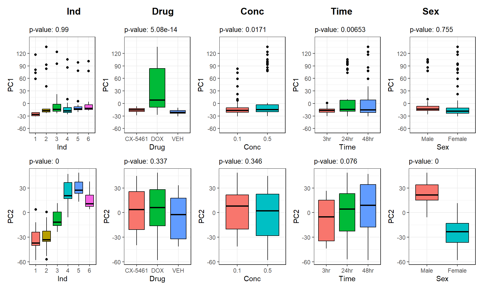
sessionInfo()R version 4.3.0 (2023-04-21 ucrt)
Platform: x86_64-w64-mingw32/x64 (64-bit)
Running under: Windows 11 x64 (build 26100)
Matrix products: default
locale:
[1] LC_COLLATE=English_United States.utf8
[2] LC_CTYPE=English_United States.utf8
[3] LC_MONETARY=English_United States.utf8
[4] LC_NUMERIC=C
[5] LC_TIME=English_United States.utf8
time zone: America/Chicago
tzcode source: internal
attached base packages:
[1] stats graphics grDevices utils datasets methods base
other attached packages:
[1] patchwork_1.3.0 ggrepel_0.9.6 tidyr_1.3.1 dplyr_1.1.4
[5] ggplot2_3.5.2 edgeR_4.0.16 limma_3.58.1
loaded via a namespace (and not attached):
[1] gtable_0.3.6 jsonlite_2.0.0 compiler_4.3.0 promises_1.3.2
[5] tidyselect_1.2.1 Rcpp_1.0.12 stringr_1.5.1 git2r_0.36.2
[9] later_1.3.2 jquerylib_0.1.4 scales_1.3.0 yaml_2.3.10
[13] fastmap_1.2.0 statmod_1.5.0 lattice_0.22-7 R6_2.6.1
[17] labeling_0.4.3 generics_0.1.3 workflowr_1.7.1 knitr_1.50
[21] tibble_3.2.1 munsell_0.5.1 rprojroot_2.0.4 bslib_0.9.0
[25] pillar_1.10.2 rlang_1.1.3 cachem_1.1.0 stringi_1.8.3
[29] httpuv_1.6.15 xfun_0.52 fs_1.6.3 sass_0.4.10
[33] cli_3.6.1 withr_3.0.2 magrittr_2.0.3 digest_0.6.34
[37] grid_4.3.0 locfit_1.5-9.12 rstudioapi_0.17.1 lifecycle_1.0.4
[41] vctrs_0.6.5 evaluate_1.0.3 glue_1.7.0 farver_2.1.2
[45] colorspace_2.1-0 purrr_1.0.4 rmarkdown_2.29 tools_4.3.0
[49] pkgconfig_2.0.3 htmltools_0.5.8.1