Revision
Last updated: 2025-10-06
Checks: 6 1
Knit directory: Paul_CX_2025/
This reproducible R Markdown analysis was created with workflowr (version 1.7.1). The Checks tab describes the reproducibility checks that were applied when the results were created. The Past versions tab lists the development history.
The R Markdown file has unstaged changes. To know which version of
the R Markdown file created these results, you’ll want to first commit
it to the Git repo. If you’re still working on the analysis, you can
ignore this warning. When you’re finished, you can run
wflow_publish to commit the R Markdown file and build the
HTML.
Great job! The global environment was empty. Objects defined in the global environment can affect the analysis in your R Markdown file in unknown ways. For reproduciblity it’s best to always run the code in an empty environment.
The command set.seed(20250129) was run prior to running
the code in the R Markdown file. Setting a seed ensures that any results
that rely on randomness, e.g. subsampling or permutations, are
reproducible.
Great job! Recording the operating system, R version, and package versions is critical for reproducibility.
Nice! There were no cached chunks for this analysis, so you can be confident that you successfully produced the results during this run.
Great job! Using relative paths to the files within your workflowr project makes it easier to run your code on other machines.
Great! You are using Git for version control. Tracking code development and connecting the code version to the results is critical for reproducibility.
The results in this page were generated with repository version 64e2d5a. See the Past versions tab to see a history of the changes made to the R Markdown and HTML files.
Note that you need to be careful to ensure that all relevant files for
the analysis have been committed to Git prior to generating the results
(you can use wflow_publish or
wflow_git_commit). workflowr only checks the R Markdown
file, but you know if there are other scripts or data files that it
depends on. Below is the status of the Git repository when the results
were generated:
Ignored files:
    Ignored:    .RData
    Ignored:    .Rhistory
    Ignored:    .Rproj.user/
    Ignored:    0.1 box.svg
    Ignored:    Rplot04.svg

Unstaged changes:
    Modified:   analysis/Revision.Rmd
Note that any generated files, e.g. HTML, png, CSS, etc., are not included in this status report because it is ok for generated content to have uncommitted changes.
These are the previous versions of the repository in which changes were
made to the R Markdown (analysis/Revision.Rmd) and HTML
(docs/Revision.html) files. If you’ve configured a remote
Git repository (see ?wflow_git_remote), click on the
hyperlinks in the table below to view the files as they were in that
past version.
| File | Version | Author | Date | Message |
|---|---|---|---|---|
| Rmd | 64e2d5a | sayanpaul01 | 2025-10-06 | Commit |
| html | 64e2d5a | sayanpaul01 | 2025-10-06 | Commit |
📌 Forest Plot: Heart Failure Risk Loci Enrichment
# 📦 Load Required Libraries
# --- Libraries ---
library(dplyr)
Warning: package 'dplyr' was built under R version 4.3.2library(tidyr)Warning: package 'tidyr' was built under R version 4.3.3library(tibble)
library(ggplot2)
# --- Step 1: Heart Failure Risk Loci (Entrez IDs) ---
entrez_ids <- c(
9709, 8882, 4023, 29959, 5496, 3992, 9415, 5308, 1026, 54437, 79068, 10221,
9031, 1187, 1952, 3705, 84722, 7273, 23293, 155382, 9531, 602, 27258, 84163,
81846, 79933, 56911, 64753, 93210, 1021, 283450, 5998, 57602, 114991, 7073,
3156, 100101267, 22996, 285025, 11080, 11124, 54810, 7531, 27241, 4774, 57794,
463, 91319, 6598, 9640, 2186, 26010, 80816, 571, 88, 51652, 64788, 90523, 2969,
7781, 80777, 10725, 23387, 817, 134728, 8842, 949, 6934, 129787, 10327, 202052,
2318, 5578, 6801, 6311, 10019, 80724, 217, 84909, 388591, 55101, 9839, 27161,
5310, 387119, 4641, 5587, 55188, 222553, 9960, 22852, 10087, 9570, 54497,
200942, 26249, 4137, 375056, 5409, 64116, 8291, 22876, 339855, 4864, 5142,
221692, 55023, 51426, 6146, 84251, 8189, 27332, 57099, 1869, 1112, 23327,
11264, 6001
)
# --- Step 2: Load DEG tables ---
deg_files <- list.files("data/DEGs/", pattern = "Toptable_.*\\.csv", full.names = TRUE)
deg_list <- lapply(deg_files, read.csv)
names(deg_list) <- gsub("Toptable_|\\.csv", "", basename(deg_files))
# --- Step 3: Fisher test function (save raw counts to table) ---
fisher_or <- function(df, sample_name) {
df <- df %>%
mutate(
DEG = adj.P.Val < 0.05,
HF_risk = Entrez_ID %in% entrez_ids
)
a <- sum(df$DEG & df$HF_risk, na.rm = TRUE)
b <- sum(df$DEG & !df$HF_risk, na.rm = TRUE)
c <- sum(!df$DEG & df$HF_risk, na.rm = TRUE)
d <- sum(!df$DEG & !df$HF_risk, na.rm = TRUE)
test <- fisher.test(matrix(c(a, b, c, d), nrow = 2))
tibble(
Sample = sample_name,
DE_Risk = a,
DE_nonRisk = b,
nonDE_Risk = c,
nonDE_nonRisk = d,
OR = unname(test$estimate),
Lower_CI = test$conf.int[1],
Upper_CI = test$conf.int[2],
Pval = test$p.value,
Stars = case_when(
test$p.value < 0.001 ~ "***",
test$p.value < 0.01 ~ "**",
test$p.value < 0.05 ~ "*",
TRUE ~ ""
)
)
}
# --- Step 4: Run Fisher tests for all DEG files ---
results <- bind_rows(mapply(fisher_or, deg_list, names(deg_list), SIMPLIFY = FALSE))
# --- Step 5: Extract metadata (Drug, Conc, Time) ---
results <- results %>%
separate(Sample, into = c("Drug","Conc","Time"), sep = "_") %>%
mutate(
Label = paste(Drug, Conc, sep = "_"),
Time = factor(Time, levels = c("3","24","48"))
)
# --- Step 6: Forest plot (clean, like before) ---
ggplot(results, aes(x = Label, y = OR, ymin = Lower_CI, ymax = Upper_CI)) +
geom_pointrange(aes(color = Pval < 0.05), size = 0.9) +
geom_text(aes(label = Stars), hjust = -0.5, size = 5) +
geom_hline(yintercept = 1, linetype = "dashed", color = "red") +
scale_color_manual(values = c("TRUE" = "blue", "FALSE" = "grey40")) +
coord_flip() +
facet_wrap(~Time, ncol = 1, scales = "free_y") +
ylim(0, 20) +
labs(
title = "Heart Failure Risk Loci Enrichment Across Conditions",
x = "Condition (Drug_Conc)",
y = "Odds Ratio (95% CI)"
) +
theme_classic(base_size = 14) +
theme(
legend.position = "none",
strip.text = element_text(face = "bold", size = 12)
)Warning: Removed 3 rows containing missing values or values outside the scale range
(`geom_segment()`).
| Version | Author | Date |
|---|---|---|
| 64e2d5a | sayanpaul01 | 2025-10-06 |
# --- Step 7: Export results with raw numbers for supplement ---
write.csv(results, "data/HF_Cardiotoxicity_ForestPlot_Data.csv", row.names = FALSE)
📌 Forest Plot: DOX Cardiotoxicity Loci Enrichment
# --- Libraries ---
library(dplyr)
library(tidyr)
library(tibble)
library(ggplot2)

# --- Step 1: Define DOX cardiotoxicity risk loci (Entrez IDs) ---
entrez_ids <- c(
  847, 873, 2064, 2878, 2944, 3038, 4846, 51196, 5880, 6687,
  7799, 4292, 5916, 3077, 51310, 9154, 64078, 5244, 10057, 10060,
  89845, 56853, 4625, 1573, 79890
)

# --- Step 2: Load DEG tables ---
deg_files <- list.files("data/DEGs/", pattern = "Toptable_.*\\.csv", full.names = TRUE)
deg_list  <- lapply(deg_files, read.csv)
names(deg_list) <- gsub("Toptable_|\\.csv", "", basename(deg_files))

# --- Step 3: Fisher test function (now saves raw counts too) ---
fisher_or <- function(df, sample_name) {
  df <- df %>%
    mutate(
      DEG = adj.P.Val < 0.05,
      DOXrisk = Entrez_ID %in% entrez_ids
    )

  a <- sum(df$DEG & df$DOXrisk, na.rm = TRUE)
  b <- sum(df$DEG & !df$DOXrisk, na.rm = TRUE)
  c <- sum(!df$DEG & df$DOXrisk, na.rm = TRUE)
  d <- sum(!df$DEG & !df$DOXrisk, na.rm = TRUE)

  test <- fisher.test(matrix(c(a, b, c, d), nrow = 2))

  tibble(
    Sample = sample_name,
    DE_Risk = a,
    DE_nonRisk = b,
    nonDE_Risk = c,
    nonDE_nonRisk = d,
    OR = unname(test$estimate),
    Lower_CI = test$conf.int[1],
    Upper_CI = test$conf.int[2],
    Pval = test$p.value,
    Stars = case_when(
      test$p.value < 0.001 ~ "***",
      test$p.value < 0.01  ~ "**",
      test$p.value < 0.05  ~ "*",
      TRUE ~ ""
    )
  )
}

# --- Step 4: Run Fisher tests for all DEG files ---
results <- bind_rows(mapply(fisher_or, deg_list, names(deg_list), SIMPLIFY = FALSE))

# --- Step 5: Extract metadata (Drug, Conc, Time) ---
results <- results %>%
  separate(Sample, into = c("Drug","Conc","Time"), sep = "_") %>%
  mutate(
    Label = paste(Drug, Conc, sep = "_"),
    Time = factor(Time, levels = c("3","24","48"))
  )

# --- Step 6: Forest plot (same clean look, 0–20 scale, stars only) ---
ggplot(results, aes(x = Label, y = OR, ymin = Lower_CI, ymax = Upper_CI)) +
  geom_pointrange(aes(color = Pval < 0.05), size = 0.9) +
  geom_text(aes(label = Stars), hjust = -0.5, size = 5) +
  geom_hline(yintercept = 1, linetype = "dashed", color = "red") +
  scale_color_manual(values = c("TRUE" = "blue", "FALSE" = "grey40")) +
  coord_flip() +
  facet_wrap(~Time, ncol = 1, scales = "free_y") +
  ylim(0, 20) +
  labs(
    title = "DOX Cardiotoxicity Loci Enrichment",
    x = "Condition (Drug_Conc)",
    y = "Odds Ratio (95% CI)"
  ) +
  theme_classic(base_size = 14) +
  theme(
    legend.position = "none",
    strip.text = element_text(face = "bold", size = 12)
  )
Warning: Removed 3 rows containing missing values or values outside the scale range
(`geom_segment()`).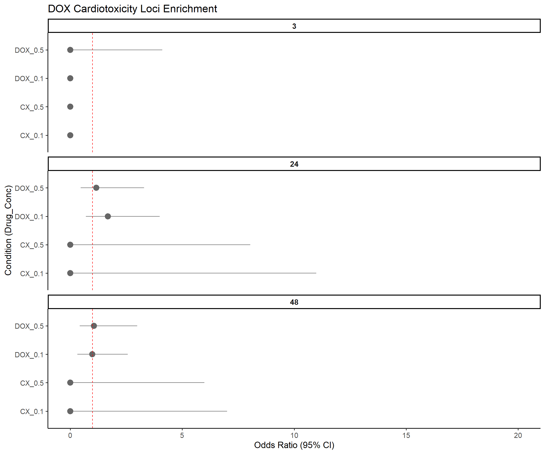
| Version | Author | Date |
|---|---|---|
| 64e2d5a | sayanpaul01 | 2025-10-06 |
# --- Step 7: Save results with raw counts for supplement ---
write.csv(results, "data/DOX_Cardiotoxicity_ForestPlot_Data.csv", row.names = FALSE)
📌 Forest Plot: AC Cardiotoxicity Loci Enrichment
# --- Libraries ---
library(dplyr)
library(tidyr)
library(tibble)
library(ggplot2)

# --- Step 1: AC Cardiotoxicity Risk Loci (Entrez IDs) ---
Entrez_IDs <- c(
  6272, 8029, 11128, 79899, 54477, 121665, 5095, 22863, 57161, 4692,
  8214, 23151, 56606, 108, 22999, 56895, 9603, 3181, 4023, 10499,
  92949, 4363, 10057, 5243, 5244, 5880, 1535, 2950, 847, 5447,
  3038, 3077, 4846, 3958, 23327, 29899, 23155, 80856, 55020, 78996,
  23262, 150383, 9620, 79730, 344595, 5066, 6251, 3482, 9588, 339416,
  7292, 55157, 87769, 23409, 720, 3107, 54535, 1590, 80059, 7991,
  57110, 8803, 323, 54826, 5916, 23371, 283337, 64078, 80010, 1933,
  10818, 51020
)

# --- Step 2: Load DEG tables ---
deg_files <- list.files("data/DEGs/", pattern = "Toptable_.*\\.csv", full.names = TRUE)
deg_list  <- lapply(deg_files, read.csv)
names(deg_list) <- gsub("Toptable_|\\.csv", "", basename(deg_files))

# --- Step 3: Fisher test function (with raw counts) ---
fisher_or <- function(df, sample_name) {
  df <- df %>%
    mutate(
      DEG = adj.P.Val < 0.05,
      AC_risk = Entrez_ID %in% Entrez_IDs
    )

  a <- sum(df$DEG & df$AC_risk, na.rm = TRUE)
  b <- sum(df$DEG & !df$AC_risk, na.rm = TRUE)
  c <- sum(!df$DEG & df$AC_risk, na.rm = TRUE)
  d <- sum(!df$DEG & !df$AC_risk, na.rm = TRUE)

  test <- fisher.test(matrix(c(a, b, c, d), nrow = 2))

  tibble(
    Sample = sample_name,
    DE_Risk = a,
    DE_nonRisk = b,
    nonDE_Risk = c,
    nonDE_nonRisk = d,
    OR = unname(test$estimate),
    Lower_CI = test$conf.int[1],
    Upper_CI = test$conf.int[2],
    Pval = test$p.value,
    Stars = case_when(
      test$p.value < 0.001 ~ "***",
      test$p.value < 0.01  ~ "**",
      test$p.value < 0.05  ~ "*",
      TRUE ~ ""
    )
  )
}

# --- Step 4: Run Fisher tests for all DEG files ---
results <- bind_rows(mapply(fisher_or, deg_list, names(deg_list), SIMPLIFY = FALSE))

# --- Step 5: Extract metadata (Drug, Conc, Time) ---
results <- results %>%
  separate(Sample, into = c("Drug","Conc","Time"), sep = "_") %>%
  mutate(
    Label = paste(Drug, Conc, sep = "_"),
    Time = factor(Time, levels = c("3","24","48"))
  )

# --- Step 6: Forest plot (scale 0–20, faceted by Time) ---
ggplot(results, aes(x = Label, y = OR, ymin = Lower_CI, ymax = Upper_CI)) +
  geom_pointrange(aes(color = Pval < 0.05), size = 0.9) +
  geom_text(aes(label = Stars), hjust = -0.5, size = 5) +
  geom_hline(yintercept = 1, linetype = "dashed", color = "red") +
  scale_color_manual(values = c("TRUE" = "blue", "FALSE" = "grey40")) +
  coord_flip() +
  facet_wrap(~Time, ncol = 1, scales = "free_y") +
  ylim(0, 20) +
  labs(
    title = "AC Cardiotoxicity Loci Enrichment Across Conditions",
    x = "Condition (Drug_Conc)",
    y = "Odds Ratio (95% CI)"
  ) +
  theme_classic(base_size = 14) +
  theme(
    legend.position = "none",
    strip.text = element_text(face = "bold", size = 12)
  )
Warning: Removed 3 rows containing missing values or values outside the scale range
(`geom_segment()`).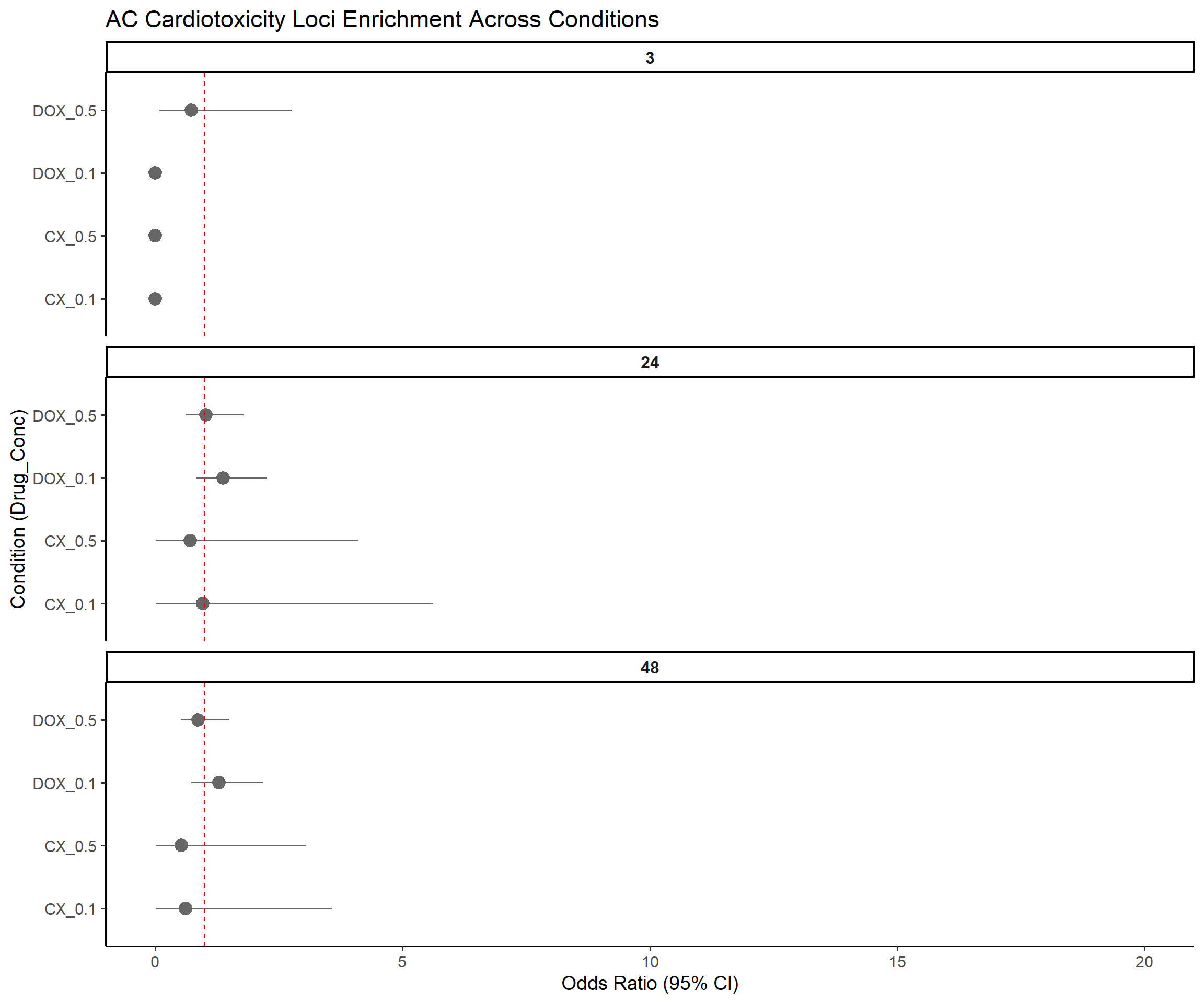
| Version | Author | Date |
|---|---|---|
| 64e2d5a | sayanpaul01 | 2025-10-06 |
# --- Step 7: Export results table (with raw numbers + OR) ---
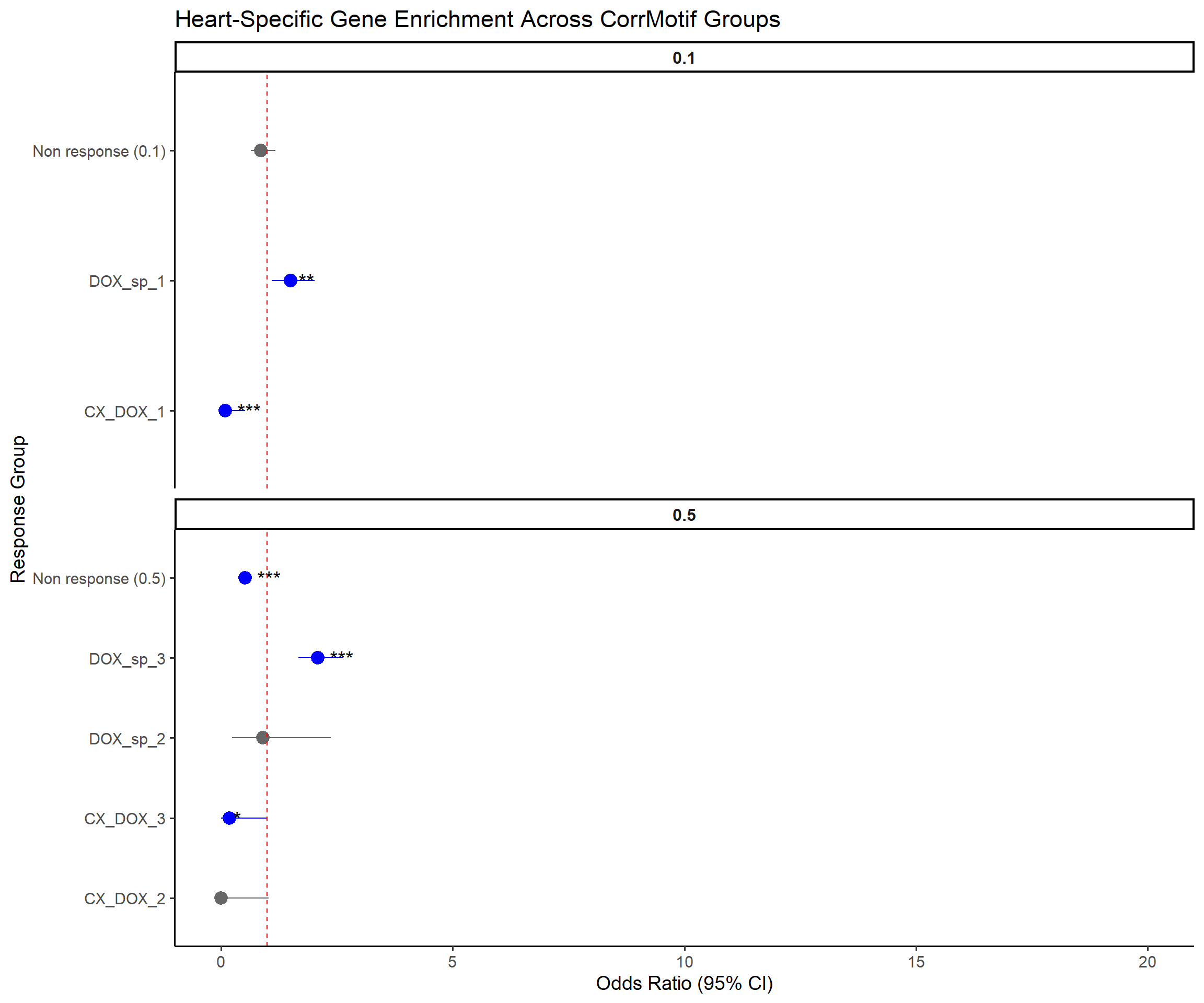
write.csv(results, "data/AC_Cardiotoxicity_ForestPlot_Data.csv", row.names = FALSE)📌 Odds Ratios for CorrMotif Groups (Heart-specific genes)
library(dplyr)
library(tidyr)
library(tibble)
library(ggplot2)
library(org.Hs.eg.db)
Warning: package 'AnnotationDbi' was built under R version 4.3.2Warning: package 'BiocGenerics' was built under R version 4.3.1Warning: package 'Biobase' was built under R version 4.3.1Warning: package 'IRanges' was built under R version 4.3.1Warning: package 'S4Vectors' was built under R version 4.3.2library(AnnotationDbi)
# --- Load Heart-Specific Genes ---
heart_genes <- read.csv("data/Human_Heart_Genes.csv", stringsAsFactors = FALSE)
heart_genes$Entrez_ID <- mapIds(
org.Hs.eg.db,
keys = heart_genes$Gene,
column = "ENTREZID",
keytype = "SYMBOL",
multiVals = "first"
)
heart_entrez_ids <- na.omit(heart_genes$Entrez_ID)
# --- Load CorrMotif Groups ---
# 0.1 µM
prob_1_0.1 <- as.character(read.csv("data/prob_1_0.1.csv")$Entrez_ID)
prob_2_0.1 <- as.character(read.csv("data/prob_2_0.1.csv")$Entrez_ID)
prob_3_0.1 <- as.character(read.csv("data/prob_3_0.1.csv")$Entrez_ID)
# 0.5 µM
prob_1_0.5 <- as.character(read.csv("data/prob_1_0.5.csv")$Entrez_ID)
prob_2_0.5 <- as.character(read.csv("data/prob_2_0.5.csv")$Entrez_ID)
prob_3_0.5 <- as.character(read.csv("data/prob_3_0.5.csv")$Entrez_ID)
prob_4_0.5 <- as.character(read.csv("data/prob_4_0.5.csv")$Entrez_ID)
prob_5_0.5 <- as.character(read.csv("data/prob_5_0.5.csv")$Entrez_ID)
# --- Annotate Groups ---
df_0.1 <- data.frame(Entrez_ID = unique(c(prob_1_0.1, prob_2_0.1, prob_3_0.1))) %>%
mutate(
Response_Group = case_when(
Entrez_ID %in% prob_1_0.1 ~ "Non response (0.1)",
Entrez_ID %in% prob_2_0.1 ~ "CX_DOX_1",
Entrez_ID %in% prob_3_0.1 ~ "DOX_sp_1"
),
Category = ifelse(Entrez_ID %in% heart_entrez_ids,
"Heart-specific Genes", "Non-Heart-specific Genes"),
Concentration = "0.1"
)
df_0.5 <- data.frame(Entrez_ID = unique(c(prob_1_0.5, prob_2_0.5, prob_3_0.5, prob_4_0.5, prob_5_0.5))) %>%
mutate(
Response_Group = case_when(
Entrez_ID %in% prob_1_0.5 ~ "Non response (0.5)",
Entrez_ID %in% prob_2_0.5 ~ "DOX_sp_2",
Entrez_ID %in% prob_3_0.5 ~ "DOX_sp_3",
Entrez_ID %in% prob_4_0.5 ~ "CX_DOX_2",
Entrez_ID %in% prob_5_0.5 ~ "CX_DOX_3"
),
Category = ifelse(Entrez_ID %in% heart_entrez_ids,
"Heart-specific Genes", "Non-Heart-specific Genes"),
Concentration = "0.5"
)
df_combined <- bind_rows(df_0.1, df_0.5)
# --- Fisher Odds Ratio Function ---
fisher_or_group <- function(df_group, df_all, group_name, conc) {
# counts in group
a <- sum(df_group$Category == "Heart-specific Genes")
b <- sum(df_group$Category == "Non-Heart-specific Genes")
# counts in rest of groups at same conc
ref <- df_all %>% filter(Response_Group != group_name)
c <- sum(ref$Category == "Heart-specific Genes")
d <- sum(ref$Category == "Non-Heart-specific Genes")
mat <- matrix(c(a, b, c, d), nrow = 2)
if (any(mat == 0)) mat <- mat + 0.5 # continuity correction
test <- fisher.test(mat)
tibble(
Response_Group = group_name,
Concentration = conc,
a = a, b = b, c = c, d = d,
OR = unname(test$estimate),
Lower_CI = test$conf.int[1],
Upper_CI = test$conf.int[2],
Pval = test$p.value,
Stars = case_when(
test$p.value < 0.001 ~ "***",
test$p.value < 0.01 ~ "**",
test$p.value < 0.05 ~ "*",
TRUE ~ ""
)
)
}
# --- Run Fisher tests safely ---
results <- list()
for (conc in unique(df_combined$Concentration)) {
conc_df <- df_combined %>% filter(Concentration == conc)
for (grp in unique(conc_df$Response_Group)) {
grp_df <- conc_df %>% filter(Response_Group == grp)
results[[paste(conc, grp)]] <- fisher_or_group(grp_df, conc_df, grp, conc)
}
}Warning in fisher.test(mat): 'x' has been rounded to integer: Mean relative
difference: 0.0001415629results <- bind_rows(results)
# --- Save Results Table ---
write.csv(results, "data/CorrMotif_HeartGenes_OddsRatios.csv", row.names = FALSE)
# --- Forest Plot ---
ggplot(results, aes(x = Response_Group, y = OR, ymin = Lower_CI, ymax = Upper_CI)) +
geom_pointrange(aes(color = Pval < 0.05), size = 0.9) +
geom_text(aes(label = Stars), hjust = -0.5, size = 5) +
geom_hline(yintercept = 1, linetype = "dashed", color = "red") +
scale_color_manual(values = c("TRUE" = "blue", "FALSE" = "grey40")) +
coord_flip() +
facet_wrap(~Concentration, ncol = 1, scales = "free_y") + # facet by concentration instead of time
ylim(0, 20) +
labs(
title = "Heart-Specific Gene Enrichment Across CorrMotif Groups",
x = "Response Group",
y = "Odds Ratio (95% CI)"
) +
theme_classic(base_size = 14) +
theme(
legend.position = "none",
strip.text = element_text(face = "bold", size = 12)
)
| Version | Author | Date |
|---|---|---|
| 64e2d5a | sayanpaul01 | 2025-10-06 |
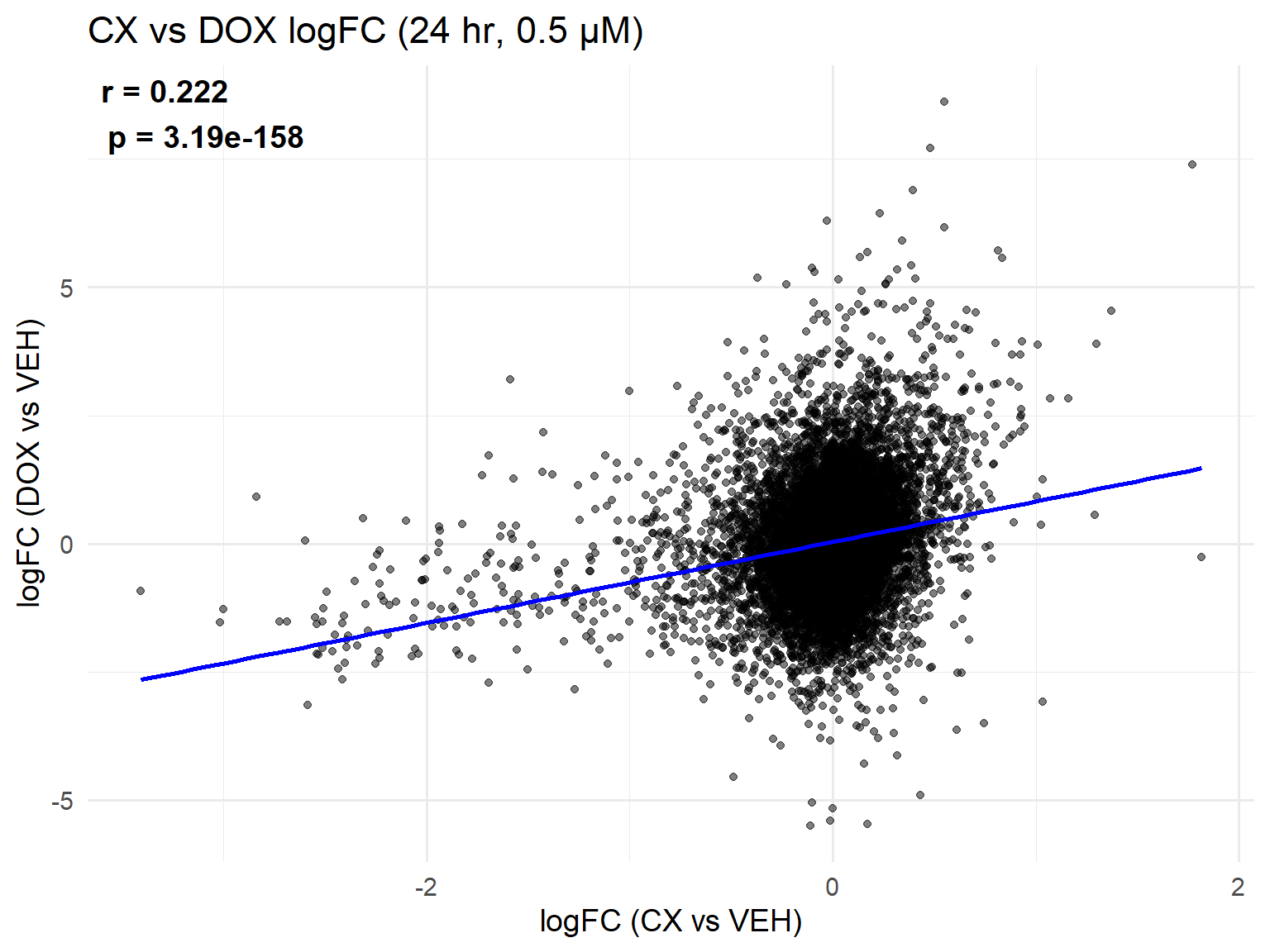
📌 Scatter Plot: DOX vs VEH vs CX vs VEH Condition: 24 hr, 0.5 µM
library(ggplot2)

# --- Load Data ---
CX_0.5_24 <- read.csv("data/DEGs/Toptable_CX_0.5_24.csv")
DOX_0.5_24 <- read.csv("data/DEGs/Toptable_DOX_0.5_24.csv")

# --- Ensure Entrez_ID is character ---
CX_0.5_24$Entrez_ID <- as.character(CX_0.5_24$Entrez_ID)
DOX_0.5_24$Entrez_ID <- as.character(DOX_0.5_24$Entrez_ID)

# --- Merge on Entrez_ID ---
merged_24h_0.5 <- merge(
  CX_0.5_24, DOX_0.5_24,
  by = "Entrez_ID", suffixes = c("_CX", "_DOX")
)

# --- Correlation ---
cor_test <- cor.test(
  merged_24h_0.5$logFC_CX,
  merged_24h_0.5$logFC_DOX,
  method = "pearson"
)

r_val <- round(cor_test$estimate, 3)
p_val <- formatC(cor_test$p.value, format = "e", digits = 2)  # scientific notation
label_text <- paste0("r = ", r_val, "\n", "p = ", p_val)

# --- Scatter Plot with fixed label placement ---
ggplot(merged_24h_0.5, aes(x = logFC_CX, y = logFC_DOX)) +
  geom_point(alpha = 0.5, color = "black") +
  geom_smooth(method = "lm", color = "blue", se = FALSE) +
  labs(
    title = "CX vs DOX logFC (24 hr, 0.5 µM)",
    x = "logFC (CX vs VEH)",
    y = "logFC (DOX vs VEH)"
  ) +
  theme_minimal(base_size = 14) +
  annotate(
    "text",
    x = -Inf, y = Inf, hjust = -0.1, vjust = 1.2,  # top-left corner inside panel
    label = label_text,
    size = 5, fontface = "bold"
  )
| Version | Author | Date |
|---|---|---|
| 64e2d5a | sayanpaul01 | 2025-10-06 |
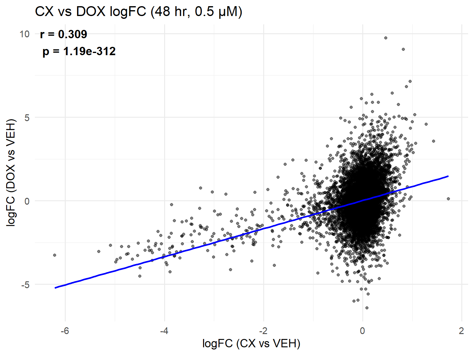
📌 Scatter Plot: DOX vs VEH vs CX vs VEH Condition: 48 hr, 0.5 µM
library(ggplot2)

# --- Load Data ---
CX_0.5_48 <- read.csv("data/DEGs/Toptable_CX_0.5_48.csv")
DOX_0.5_48 <- read.csv("data/DEGs/Toptable_DOX_0.5_48.csv")

# --- Ensure Entrez_ID is character ---
CX_0.5_48$Entrez_ID <- as.character(CX_0.5_48$Entrez_ID)
DOX_0.5_48$Entrez_ID <- as.character(DOX_0.5_48$Entrez_ID)

# --- Merge on Entrez_ID ---
merged_48h_0.5 <- merge(
  CX_0.5_48, DOX_0.5_48,
  by = "Entrez_ID", suffixes = c("_CX", "_DOX")
)


# --- Correlation ---
cor_test <- cor.test(
  merged_48h_0.5$logFC_CX,
  merged_48h_0.5$logFC_DOX,
  method = "pearson"
)

r_val <- round(cor_test$estimate, 3)
p_val <- formatC(cor_test$p.value, format = "e", digits = 2)  # scientific notation
label_text <- paste0("r = ", r_val, "\n", "p = ", p_val)

# --- Scatter Plot with fixed label placement ---
ggplot(merged_48h_0.5, aes(x = logFC_CX, y = logFC_DOX)) +
  geom_point(alpha = 0.5, color = "black") +
  geom_smooth(method = "lm", color = "blue", se = FALSE) +
  labs(
    title = "CX vs DOX logFC (48 hr, 0.5 µM)",
    x = "logFC (CX vs VEH)",
    y = "logFC (DOX vs VEH)"
  ) +
  theme_minimal(base_size = 14) +
  annotate(
    "text",
    x = -Inf, y = Inf, hjust = -0.1, vjust = 1.2,  # top-left corner inside panel
    label = label_text,
    size = 5, fontface = "bold"
  )
| Version | Author | Date |
|---|---|---|
| 64e2d5a | sayanpaul01 | 2025-10-06 |
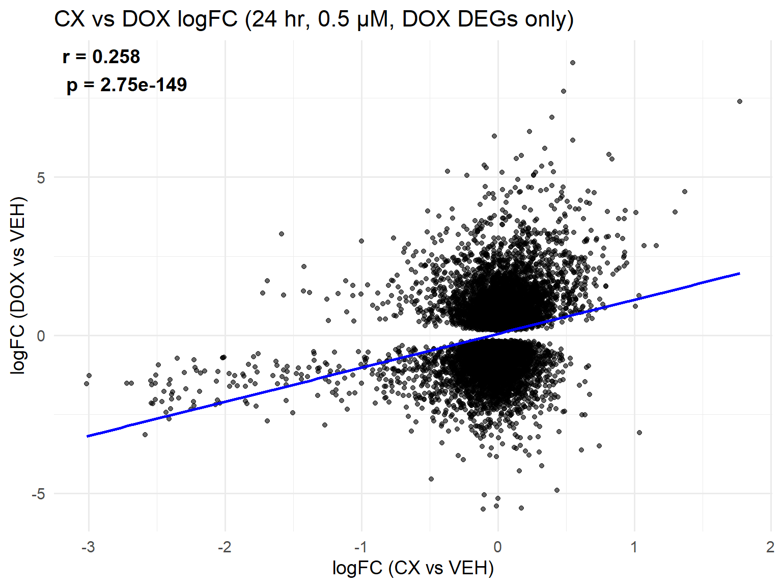
📌 Scatter Plot: DOX vs VEH vs CX vs VEH Condition: 24 hr, 0.5 µM (DOX DEGs only)
library(ggplot2)

# --- Load Data ---
CX_0.5_24 <- read.csv("data/DEGs/Toptable_CX_0.5_24.csv")
DOX_0.5_24 <- read.csv("data/DEGs/Toptable_DOX_0.5_24.csv")

# --- Ensure Entrez_ID is character ---
CX_0.5_24$Entrez_ID <- as.character(CX_0.5_24$Entrez_ID)
DOX_0.5_24$Entrez_ID <- as.character(DOX_0.5_24$Entrez_ID)

# --- Extract DEGs from DOX (adj.P.Val < 0.05) ---
dox_degs <- DOX_0.5_24$Entrez_ID[DOX_0.5_24$adj.P.Val < 0.05]

# --- Merge CX & DOX, filter for DOX DEGs only ---
merged_24h_0.5 <- merge(
  CX_0.5_24, DOX_0.5_24,
  by = "Entrez_ID", suffixes = c("_CX", "_DOX")
)

merged_24h_0.5 <- merged_24h_0.5[merged_24h_0.5$Entrez_ID %in% dox_degs, ]

# --- Correlation ---
cor_test <- cor.test(
  merged_24h_0.5$logFC_CX,
  merged_24h_0.5$logFC_DOX,
  method = "pearson"
)

r_val <- round(cor_test$estimate, 3)
p_val <- formatC(cor_test$p.value, format = "e", digits = 2)
label_text <- paste0("r = ", r_val, "\n", "p = ", p_val)

# --- Scatter Plot ---
ggplot(merged_24h_0.5, aes(x = logFC_CX, y = logFC_DOX)) +
  geom_point(alpha = 0.6, color = "black") +
  geom_smooth(method = "lm", color = "blue", se = FALSE) +
  labs(
    title = "CX vs DOX logFC (24 hr, 0.5 µM, DOX DEGs only)",
    x = "logFC (CX vs VEH)",
    y = "logFC (DOX vs VEH)"
  ) +
  theme_minimal(base_size = 14) +
  annotate(
    "text",
    x = -Inf, y = Inf,
    hjust = -0.1, vjust = 1.2,
    label = label_text,
    size = 5, fontface = "bold"
  )
| Version | Author | Date |
|---|---|---|
| 64e2d5a | sayanpaul01 | 2025-10-06 |
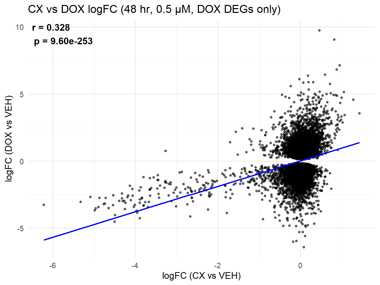
📌 Scatter Plot: DOX vs VEH vs CX vs VEH Condition: 48 hr, 0.5 µM (DOX DEGs only)
library(ggplot2)

# --- Load Data ---
CX_0.5_48 <- read.csv("data/DEGs/Toptable_CX_0.5_48.csv")
DOX_0.5_48 <- read.csv("data/DEGs/Toptable_DOX_0.5_48.csv")

# --- Ensure Entrez_ID is character ---
CX_0.5_48$Entrez_ID <- as.character(CX_0.5_48$Entrez_ID)
DOX_0.5_48$Entrez_ID <- as.character(DOX_0.5_48$Entrez_ID)

# --- Extract DEGs from DOX (adj.P.Val < 0.05) ---
dox_degs <- DOX_0.5_48$Entrez_ID[DOX_0.5_48$adj.P.Val < 0.05]

# --- Merge CX & DOX, filter for DOX DEGs only ---
merged_48h_0.5 <- merge(
  CX_0.5_48, DOX_0.5_48,
  by = "Entrez_ID", suffixes = c("_CX", "_DOX")
)

merged_48h_0.5 <- merged_48h_0.5[merged_48h_0.5$Entrez_ID %in% dox_degs, ]

# --- Correlation ---
cor_test <- cor.test(
  merged_48h_0.5$logFC_CX,
  merged_48h_0.5$logFC_DOX,
  method = "pearson"
)

r_val <- round(cor_test$estimate, 3)
p_val <- formatC(cor_test$p.value, format = "e", digits = 2)
label_text <- paste0("r = ", r_val, "\n", "p = ", p_val)

# --- Scatter Plot ---
ggplot(merged_48h_0.5, aes(x = logFC_CX, y = logFC_DOX)) +
  geom_point(alpha = 0.6, color = "black") +
  geom_smooth(method = "lm", color = "blue", se = FALSE) +
  labs(
    title = "CX vs DOX logFC (48 hr, 0.5 µM, DOX DEGs only)",
    x = "logFC (CX vs VEH)",
    y = "logFC (DOX vs VEH)"
  ) +
  theme_minimal(base_size = 14) +
  annotate(
    "text",
    x = -Inf, y = Inf,
    hjust = -0.1, vjust = 1.2,
    label = label_text,
    size = 5, fontface = "bold"
  )
| Version | Author | Date |
|---|---|---|
| 64e2d5a | sayanpaul01 | 2025-10-06 |
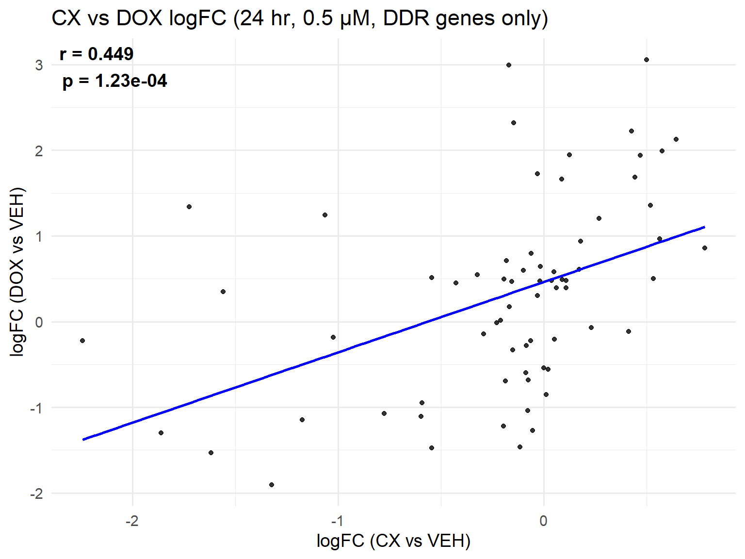
📌 Scatter Plot: DOX vs VEH vs CX vs VEH Condition: 24 hr, 0.5 µM (DDR genes only, cleaned set)
library(ggplot2)
library(dplyr)

# --- DDR gene set ---
entrez_ids <- c(
  10111, 1017, 1019, 1020, 1021, 1026, 1027, 10912, 11011, 1111,
  11200, 1385, 1643, 1647, 1869, 207, 2177, 25, 27113, 27244,
  3014, 317, 355, 4193, 4292, 4361, 4609, 4616, 4683, 472, 50484,
  5366, 5371, 54205, 545, 55367, 5591, 581, 5810, 5883, 5884,
  5888, 5893, 5925, 595, 5981, 6118, 637, 672, 7157, 7799,
  8243, 836, 841, 84126, 842, 8795, 891, 894, 896, 898,
  9133, 9134, 983, 9874, 993, 995, 5916
) %>% as.character()

# --- Load Data ---
CX_0.5_24 <- read.csv("data/DEGs/Toptable_CX_0.5_24.csv")
DOX_0.5_24 <- read.csv("data/DEGs/Toptable_DOX_0.5_24.csv")

CX_0.5_24$Entrez_ID <- as.character(CX_0.5_24$Entrez_ID)
DOX_0.5_24$Entrez_ID <- as.character(DOX_0.5_24$Entrez_ID)

# --- Merge and filter for DDR genes ---
merged_ddr_24h_0.5 <- merge(
  CX_0.5_24, DOX_0.5_24,
  by = "Entrez_ID", suffixes = c("_CX", "_DOX")
)

merged_ddr_24h_0.5 <- merged_ddr_24h_0.5 %>%
  filter(Entrez_ID %in% entrez_ids)

# --- Correlation ---
cor_test <- cor.test(
  merged_ddr_24h_0.5$logFC_CX,
  merged_ddr_24h_0.5$logFC_DOX,
  method = "pearson"
)

r_val <- round(cor_test$estimate, 3)
p_val <- formatC(cor_test$p.value, format = "e", digits = 2)
label_text <- paste0("r = ", r_val, "\n", "p = ", p_val)

# --- Scatter Plot ---
ggplot(merged_ddr_24h_0.5, aes(x = logFC_CX, y = logFC_DOX)) +
  geom_point(alpha = 0.8, color = "black") +
  geom_smooth(method = "lm", color = "blue", se = FALSE) +
  labs(
    title = "CX vs DOX logFC (24 hr, 0.5 µM, DDR genes only)",
    x = "logFC (CX vs VEH)",
    y = "logFC (DOX vs VEH)"
  ) +
  theme_minimal(base_size = 14) +
  annotate(
    "text",
    x = -Inf, y = Inf,
    hjust = -0.1, vjust = 1.2,
    label = label_text,
    size = 5, fontface = "bold"
  )
| Version | Author | Date |
|---|---|---|
| 64e2d5a | sayanpaul01 | 2025-10-06 |
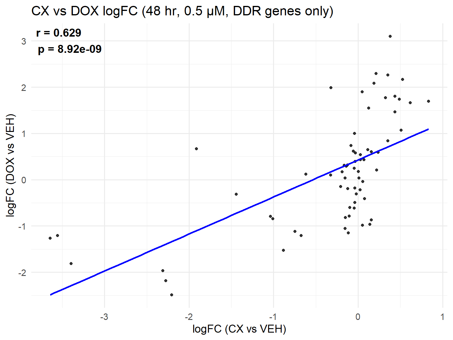
📌 Scatter Plot: DOX vs VEH vs CX vs VEH Condition: 48 hr, 0.5 µM (DDR genes only)
library(ggplot2)
library(dplyr)

# --- DDR gene set (Entrez IDs) ---
entrez_ids <- c(
  10111, 1017, 1019, 1020, 1021, 1026, 1027, 10912, 11011, 1111,
  11200, 1385, 1643, 1647, 1869, 207, 2177, 25, 27113, 27244,
  3014, 317, 355, 4193, 4292, 4361, 4609, 4616, 4683, 472, 50484,
  5366, 5371, 54205, 545, 55367, 5591, 581, 5810, 5883, 5884,
  5888, 5893, 5925, 595, 5981, 6118, 637, 672, 7157, 7799,
  8243, 836, 841, 84126, 842, 8795, 891, 894, 896, 898,
  9133, 9134, 983, 9874, 993, 995, 5916
) %>% as.character()

# --- Load Data ---
CX_0.5_48 <- read.csv("data/DEGs/Toptable_CX_0.5_48.csv")
DOX_0.5_48 <- read.csv("data/DEGs/Toptable_DOX_0.5_48.csv")

CX_0.5_48$Entrez_ID <- as.character(CX_0.5_48$Entrez_ID)
DOX_0.5_48$Entrez_ID <- as.character(DOX_0.5_48$Entrez_ID)

# --- Merge and filter for DDR genes ---
merged_ddr_48h_0.5 <- merge(
  CX_0.5_48, DOX_0.5_48,
  by = "Entrez_ID", suffixes = c("_CX", "_DOX")
)

merged_ddr_48h_0.5 <- merged_ddr_48h_0.5 %>%
  filter(Entrez_ID %in% entrez_ids)

# --- Correlation ---
cor_test <- cor.test(
  merged_ddr_48h_0.5$logFC_CX,
  merged_ddr_48h_0.5$logFC_DOX,
  method = "pearson"
)

r_val <- round(cor_test$estimate, 3)
p_val <- formatC(cor_test$p.value, format = "e", digits = 2)
label_text <- paste0("r = ", r_val, "\n", "p = ", p_val)

# --- Scatter Plot ---
ggplot(merged_ddr_48h_0.5, aes(x = logFC_CX, y = logFC_DOX)) +
  geom_point(alpha = 0.8, color = "black") +
  geom_smooth(method = "lm", color = "blue", se = FALSE) +
  labs(
    title = "CX vs DOX logFC (48 hr, 0.5 µM, DDR genes only)",
    x = "logFC (CX vs VEH)",
    y = "logFC (DOX vs VEH)"
  ) +
  theme_minimal(base_size = 14) +
  annotate(
    "text",
    x = -Inf, y = Inf,
    hjust = -0.1, vjust = 1.2,
    label = label_text,
    size = 5, fontface = "bold"
  )
| Version | Author | Date |
|---|---|---|
| 64e2d5a | sayanpaul01 | 2025-10-06 |
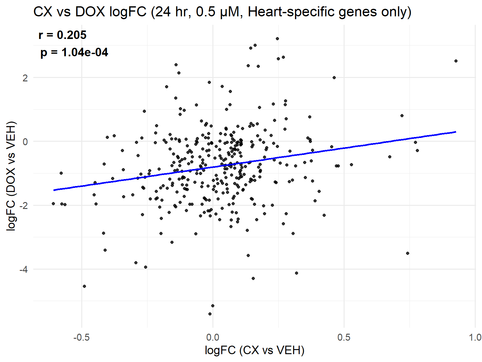
📌 Scatter Plot: DOX vs VEH vs CX vs VEH Condition: 24 hr, 0.5 µM (Heart-specific genes only)
library(dplyr)
library(ggplot2)
library(org.Hs.eg.db)
library(AnnotationDbi)

# --- Load Heart-Specific Genes ---
heart_genes <- read.csv("data/Human_Heart_Genes.csv", stringsAsFactors = FALSE)
heart_genes$Entrez_ID <- mapIds(
  org.Hs.eg.db,
  keys = heart_genes$Gene,
  column = "ENTREZID",
  keytype = "SYMBOL",
  multiVals = "first"
)
heart_entrez_ids <- na.omit(heart_genes$Entrez_ID) %>% as.character()

# --- Load DEG Data ---
CX_0.5_24 <- read.csv("data/DEGs/Toptable_CX_0.5_24.csv")
DOX_0.5_24 <- read.csv("data/DEGs/Toptable_DOX_0.5_24.csv")

CX_0.5_24$Entrez_ID <- as.character(CX_0.5_24$Entrez_ID)
DOX_0.5_24$Entrez_ID <- as.character(DOX_0.5_24$Entrez_ID)

# --- Merge and filter for heart-specific genes ---
merged_heart_24h_0.5 <- merge(
  CX_0.5_24, DOX_0.5_24,
  by = "Entrez_ID", suffixes = c("_CX", "_DOX")
)

merged_heart_24h_0.5 <- merged_heart_24h_0.5 %>%
  filter(Entrez_ID %in% heart_entrez_ids)

# --- Correlation ---
cor_test <- cor.test(
  merged_heart_24h_0.5$logFC_CX,
  merged_heart_24h_0.5$logFC_DOX,
  method = "pearson"
)

r_val <- round(cor_test$estimate, 3)
p_val <- formatC(cor_test$p.value, format = "e", digits = 2)
label_text <- paste0("r = ", r_val, "\n", "p = ", p_val)

# --- Scatter Plot ---
ggplot(merged_heart_24h_0.5, aes(x = logFC_CX, y = logFC_DOX)) +
  geom_point(alpha = 0.8, color = "black") +
  geom_smooth(method = "lm", color = "blue", se = FALSE) +
  labs(
    title = "CX vs DOX logFC (24 hr, 0.5 µM, Heart-specific genes only)",
    x = "logFC (CX vs VEH)",
    y = "logFC (DOX vs VEH)"
  ) +
  theme_minimal(base_size = 14) +
  annotate(
    "text",
    x = -Inf, y = Inf,
    hjust = -0.1, vjust = 1.2,
    label = label_text,
    size = 5, fontface = "bold"
  )
| Version | Author | Date |
|---|---|---|
| 64e2d5a | sayanpaul01 | 2025-10-06 |
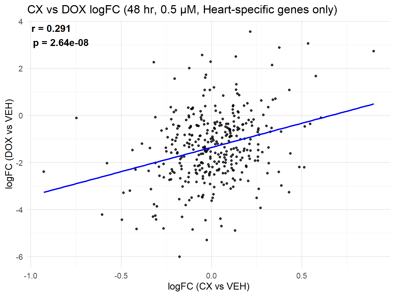
📌 Scatter Plot: DOX vs VEH vs CX vs VEH Condition: 48 hr, 0.5 µM (Heart-specific genes only)
library(dplyr)
library(ggplot2)
library(org.Hs.eg.db)
library(AnnotationDbi)

# --- Load Heart-Specific Genes ---
heart_genes <- read.csv("data/Human_Heart_Genes.csv", stringsAsFactors = FALSE)
heart_genes$Entrez_ID <- mapIds(
  org.Hs.eg.db,
  keys = heart_genes$Gene,
  column = "ENTREZID",
  keytype = "SYMBOL",
  multiVals = "first"
)
heart_entrez_ids <- na.omit(heart_genes$Entrez_ID) %>% as.character()

# --- Load DEG Data ---
CX_0.5_48 <- read.csv("data/DEGs/Toptable_CX_0.5_48.csv")
DOX_0.5_48 <- read.csv("data/DEGs/Toptable_DOX_0.5_48.csv")

CX_0.5_48$Entrez_ID <- as.character(CX_0.5_48$Entrez_ID)
DOX_0.5_48$Entrez_ID <- as.character(DOX_0.5_48$Entrez_ID)

# --- Merge and filter for heart-specific genes ---
merged_heart_48h_0.5 <- merge(
  CX_0.5_48, DOX_0.5_48,
  by = "Entrez_ID", suffixes = c("_CX", "_DOX")
)

merged_heart_48h_0.5 <- merged_heart_48h_0.5 %>%
  filter(Entrez_ID %in% heart_entrez_ids)

# --- Correlation ---
cor_test <- cor.test(
  merged_heart_48h_0.5$logFC_CX,
  merged_heart_48h_0.5$logFC_DOX,
  method = "pearson"
)

r_val <- round(cor_test$estimate, 3)
p_val <- formatC(cor_test$p.value, format = "e", digits = 2)
label_text <- paste0("r = ", r_val, "\n", "p = ", p_val)

# --- Scatter Plot ---
ggplot(merged_heart_48h_0.5, aes(x = logFC_CX, y = logFC_DOX)) +
  geom_point(alpha = 0.8, color = "black") +
  geom_smooth(method = "lm", color = "blue", se = FALSE) +
  labs(
    title = "CX vs DOX logFC (48 hr, 0.5 µM, Heart-specific genes only)",
    x = "logFC (CX vs VEH)",
    y = "logFC (DOX vs VEH)"
  ) +
  theme_minimal(base_size = 14) +
  annotate(
    "text",
    x = -Inf, y = Inf,
    hjust = -0.1, vjust = 1.2,
    label = label_text,
    size = 5, fontface = "bold"
  )
| Version | Author | Date |
|---|---|---|
| 64e2d5a | sayanpaul01 | 2025-10-06 |
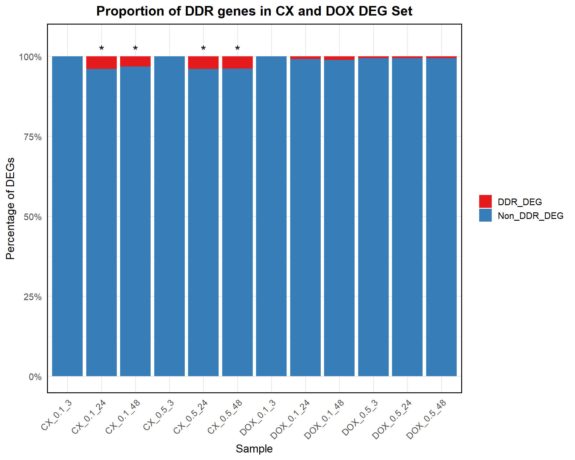
📌 Proportion of DDR DEGs in CX and DOX treated samples
# ------------------ Load Libraries ------------------
library(tidyverse)
Warning: package 'tidyverse' was built under R version 4.3.2Warning: package 'readr' was built under R version 4.3.3Warning: package 'purrr' was built under R version 4.3.3Warning: package 'stringr' was built under R version 4.3.2Warning: package 'lubridate' was built under R version 4.3.3library(org.Hs.eg.db)
# ------------------ Define DDR Gene Set ------------------
ddr_entrez <- c(
10111, 1017, 1019, 1020, 1021, 1026, 1027, 10912, 11011, 1111,
11200, 1385, 1643, 1647, 1869, 207, 2177, 25, 27113, 27244,
3014, 317, 355, 4193, 4292, 4361, 4609, 4616, 4683, 472, 50484,
5366, 5371, 54205, 545, 55367, 5591, 581, 5810, 5883, 5884,
5888, 5893, 5925, 595, 5981, 6118, 637, 672, 7157, 7799,
8243, 836, 841, 84126, 842, 8795, 891, 894, 896, 898,
9133, 9134, 983, 9874, 993, 995, 5916
) %>% as.character()
# ------------------ Load DEG Data ------------------
deg_list <- list(
"CX_0.1_3" = read.csv("data/DEGs/Toptable_CX_0.1_3.csv"),
"CX_0.1_24" = read.csv("data/DEGs/Toptable_CX_0.1_24.csv"),
"CX_0.1_48" = read.csv("data/DEGs/Toptable_CX_0.1_48.csv"),
"CX_0.5_3" = read.csv("data/DEGs/Toptable_CX_0.5_3.csv"),
"CX_0.5_24" = read.csv("data/DEGs/Toptable_CX_0.5_24.csv"),
"CX_0.5_48" = read.csv("data/DEGs/Toptable_CX_0.5_48.csv"),
"DOX_0.1_3" = read.csv("data/DEGs/Toptable_DOX_0.1_3.csv"),
"DOX_0.1_24" = read.csv("data/DEGs/Toptable_DOX_0.1_24.csv"),
"DOX_0.1_48" = read.csv("data/DEGs/Toptable_DOX_0.1_48.csv"),
"DOX_0.5_3" = read.csv("data/DEGs/Toptable_DOX_0.5_3.csv"),
"DOX_0.5_24" = read.csv("data/DEGs/Toptable_DOX_0.5_24.csv"),
"DOX_0.5_48" = read.csv("data/DEGs/Toptable_DOX_0.5_48.csv")
)
# ------------------ Compute Proportions ------------------
proportion_data <- map_dfr(names(deg_list), function(sample) {
sig_df <- deg_list[[sample]] %>% filter(adj.P.Val < 0.05)
sample_degs <- unique(as.character(sig_df$Entrez_ID))
yes <- sum(sample_degs %in% ddr_entrez)
no <- length(sample_degs) - yes
data.frame(
Sample = sample,
Category = c("DDR_DEG", "Non_DDR_DEG"),
Count = c(yes, no)
)
}) %>%
group_by(Sample) %>%
mutate(Proportion = Count / sum(Count) * 100)
# ------------------ Set Order ------------------
proportion_data$Sample <- factor(proportion_data$Sample, levels = c(
"CX_0.1_3", "CX_0.1_24", "CX_0.1_48",
"CX_0.5_3", "CX_0.5_24", "CX_0.5_48",
"DOX_0.1_3", "DOX_0.1_24", "DOX_0.1_48",
"DOX_0.5_3", "DOX_0.5_24", "DOX_0.5_48"
))
proportion_data$Category <- factor(proportion_data$Category,
levels = c("DDR_DEG", "Non_DDR_DEG"))
# ------------------ Statistical Testing (CX vs DOX) ------------------
matched_pairs <- list(
"0.1_3" = c("CX_0.1_3", "DOX_0.1_3"),
"0.1_24" = c("CX_0.1_24", "DOX_0.1_24"),
"0.1_48" = c("CX_0.1_48", "DOX_0.1_48"),
"0.5_3" = c("CX_0.5_3", "DOX_0.5_3"),
"0.5_24" = c("CX_0.5_24", "DOX_0.5_24"),
"0.5_48" = c("CX_0.5_48", "DOX_0.5_48")
)
test_results <- map_dfr(names(matched_pairs), function(label) {
cx <- matched_pairs[[label]][1]
dox <- matched_pairs[[label]][2]
cx_df <- deg_list[[cx]] %>% filter(adj.P.Val < 0.05)
dox_df <- deg_list[[dox]] %>% filter(adj.P.Val < 0.05)
a1 <- sum(cx_df$Entrez_ID %in% ddr_entrez)
b1 <- nrow(cx_df) - a1
a2 <- sum(dox_df$Entrez_ID %in% ddr_entrez)
b2 <- nrow(dox_df) - a2
mat <- matrix(c(a1, b1, a2, b2), nrow = 2, byrow = TRUE)
test <- if (min(mat) < 5) fisher.test(mat) else chisq.test(mat)
data.frame(
Comparison = label,
CX_sample = cx,
DOX_sample = dox,
a1 = a1, b1 = b1, a2 = a2, b2 = b2,
P_value = test$p.value,
Stars = ifelse(test$p.value < 0.05, "*", "")
)
})Warning in chisq.test(mat): Chi-squared approximation may be incorrectWarning in chisq.test(mat): Chi-squared approximation may be incorrect
Warning in chisq.test(mat): Chi-squared approximation may be incorrect
Warning in chisq.test(mat): Chi-squared approximation may be incorrectwrite.csv(test_results, "data/DDR_DEG_overlap_stats.csv", row.names = FALSE)
# ------------------ Plot ------------------
ggplot(proportion_data, aes(x = Sample, y = Proportion, fill = Category)) +
geom_bar(stat = "identity") +
geom_text(
data = test_results %>% filter(Stars != "") %>%
mutate(Sample = CX_sample, y_pos = 102),
aes(x = Sample, y = y_pos, label = Stars),
inherit.aes = FALSE, size = 6
) +
scale_fill_manual(values = c("DDR_DEG" = "#e41a1c", "Non_DDR_DEG" = "#377eb8")) +
scale_y_continuous(labels = scales::percent_format(scale = 1), limits = c(0, 105)) +
labs(
title = "Proportion of DDR genes in CX and DOX DEG Set",
x = "Sample",
y = "Percentage of DEGs",
fill = "Category"
) +
theme_minimal(base_size = 14) +
theme(
axis.text.x = element_text(angle = 45, hjust = 1),
plot.title = element_text(hjust = 0.5, face = "bold"),
legend.title = element_blank(),
panel.border = element_rect(color = "black", fill = NA, linewidth = 1)
)
| Version | Author | Date |
|---|---|---|
| 64e2d5a | sayanpaul01 | 2025-10-06 |
📌 Forest Plot: DDR Gene Enrichment
# --- Libraries ---
library(dplyr)
library(tidyr)
library(tibble)
library(ggplot2)

# --- Step 1: DDR Gene Set (Entrez IDs) ---
ddr_entrez <- c(
  10111, 1017, 1019, 1020, 1021, 1026, 1027, 10912, 11011, 1111,
  11200, 1385, 1643, 1647, 1869, 207, 2177, 25, 27113, 27244,
  3014, 317, 355, 4193, 4292, 4361, 4609, 4616, 4683, 472, 50484,
  5366, 5371, 54205, 545, 55367, 5591, 581, 5810, 5883, 5884,
  5888, 5893, 5925, 595, 5981, 6118, 637, 672, 7157, 7799,
  8243, 836, 841, 84126, 842, 8795, 891, 894, 896, 898,
  9133, 9134, 983, 9874, 993, 995, 5916
) %>% as.character()

# --- Step 2: Load DEG tables ---
deg_files <- list.files("data/DEGs/", pattern = "Toptable_.*\\.csv", full.names = TRUE)
deg_list  <- lapply(deg_files, read.csv)
names(deg_list) <- gsub("Toptable_|\\.csv", "", basename(deg_files))

# --- Step 3: Fisher test function (save raw counts too) ---
fisher_or <- function(df, sample_name) {
  df <- df %>%
    mutate(
      DEG = adj.P.Val < 0.05,
      DDR_gene = Entrez_ID %in% ddr_entrez
    )

  a <- sum(df$DEG & df$DDR_gene, na.rm = TRUE)   # DDR genes among DEGs
  b <- sum(df$DEG & !df$DDR_gene, na.rm = TRUE)  # Non-DDR among DEGs
  c <- sum(!df$DEG & df$DDR_gene, na.rm = TRUE)  # DDR genes not DEGs
  d <- sum(!df$DEG & !df$DDR_gene, na.rm = TRUE) # Non-DDR not DEGs

  test <- fisher.test(matrix(c(a, b, c, d), nrow = 2))

  tibble(
    Sample = sample_name,
    DE_DDR = a,
    DE_nonDDR = b,
    nonDE_DDR = c,
    nonDE_nonDDR = d,
    OR = unname(test$estimate),
    Lower_CI = test$conf.int[1],
    Upper_CI = test$conf.int[2],
    Pval = test$p.value,
    Stars = case_when(
      test$p.value < 0.001 ~ "***",
      test$p.value < 0.01  ~ "**",
      test$p.value < 0.05  ~ "*",
      TRUE ~ ""
    )
  )
}

# --- Step 4: Run Fisher tests for all DEG files ---
results <- bind_rows(mapply(fisher_or, deg_list, names(deg_list), SIMPLIFY = FALSE))

# --- Step 5: Extract metadata (Drug, Conc, Time) ---
results <- results %>%
  separate(Sample, into = c("Drug","Conc","Time"), sep = "_") %>%
  mutate(
    Label = paste(Drug, Conc, sep = "_"),
    Time = factor(Time, levels = c("3","24","48")) # enforce order
  )

# --- Step 6: Forest Plot ---
ggplot(results, aes(x = Label, y = OR, ymin = Lower_CI, ymax = Upper_CI)) +
  geom_pointrange(color = "black", size = 0.9) +
  geom_text(aes(label = Stars), hjust = -0.5, size = 5) +
  geom_hline(yintercept = 1, linetype = "dashed", color = "red") +
  coord_flip() +
  facet_wrap(~Time, ncol = 1, scales = "free_y") +
  ylim(0, 20) +   # fixed OR scale
  labs(
    title = "DDR Gene Enrichment Across Conditions",
    x = "Condition (Drug_Conc)",
    y = "Odds Ratio (95% CI)"
  ) +
  theme_classic(base_size = 14) +
  theme(
    legend.position = "none",
    strip.text = element_text(face = "bold", size = 12)
  )
Warning: Removed 3 rows containing missing values or values outside the scale range
(`geom_segment()`).Warning: Removed 1 row containing missing values or values outside the scale range
(`geom_segment()`).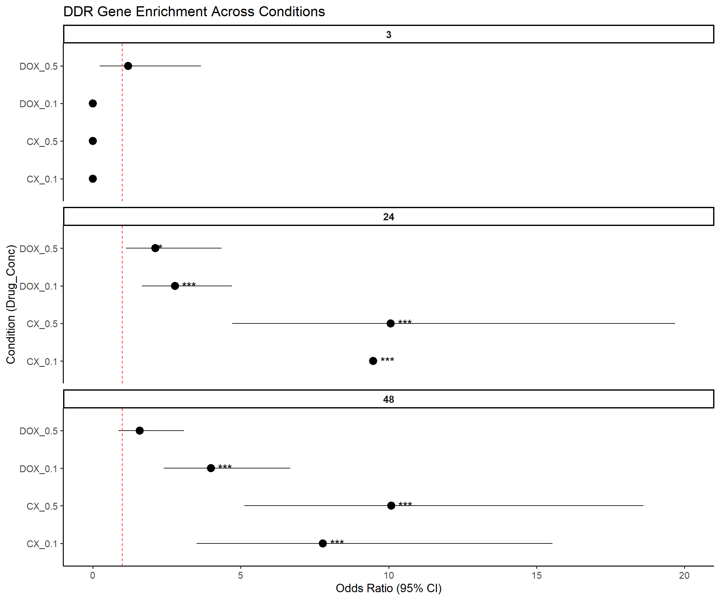
| Version | Author | Date |
|---|---|---|
| 64e2d5a | sayanpaul01 | 2025-10-06 |
# --- Step 7: Export results (with raw numbers) ---
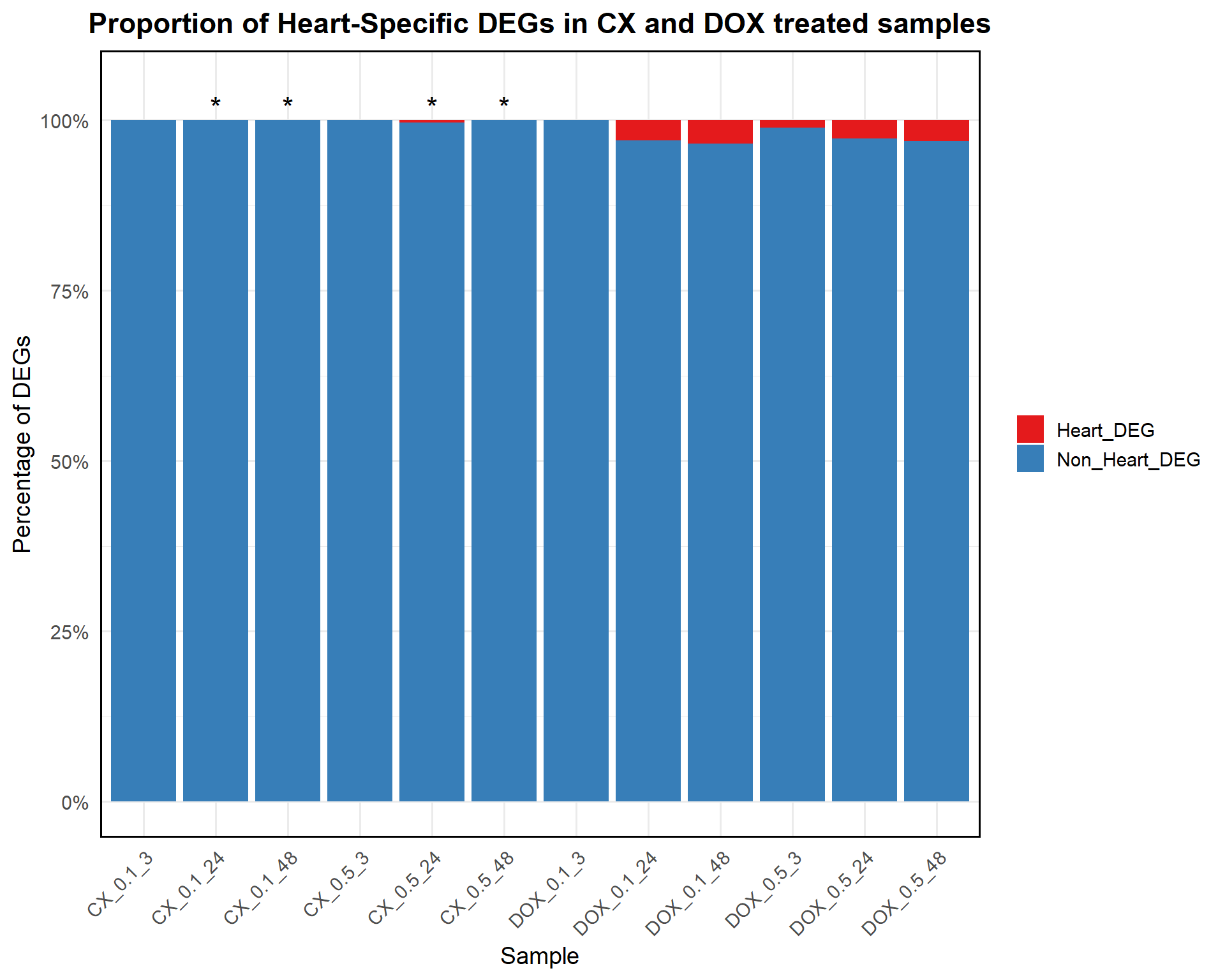
write.csv(results, "data/DDR_ForestPlot_Data.csv", row.names = FALSE)📌 Proportion of Heart-Specific DEGs in CX and DOX treated samples
# ------------------ Load Libraries ------------------
library(tidyverse)
library(org.Hs.eg.db)
library(AnnotationDbi)

# ------------------ Load Heart-Specific Genes ------------------
heart_genes <- read.csv("data/Human_Heart_Genes.csv", stringsAsFactors = FALSE)
heart_genes$Entrez_ID <- mapIds(
  org.Hs.eg.db,
  keys = heart_genes$Gene,
  column = "ENTREZID",
  keytype = "SYMBOL",
  multiVals = "first"
)
heart_entrez_ids <- na.omit(heart_genes$Entrez_ID) %>% as.character()

# ------------------ Load DEG Data ------------------
deg_list <- list(
  "CX_0.1_3"   = read.csv("data/DEGs/Toptable_CX_0.1_3.csv"),
  "CX_0.1_24"  = read.csv("data/DEGs/Toptable_CX_0.1_24.csv"),
  "CX_0.1_48"  = read.csv("data/DEGs/Toptable_CX_0.1_48.csv"),
  "CX_0.5_3"   = read.csv("data/DEGs/Toptable_CX_0.5_3.csv"),
  "CX_0.5_24"  = read.csv("data/DEGs/Toptable_CX_0.5_24.csv"),
  "CX_0.5_48"  = read.csv("data/DEGs/Toptable_CX_0.5_48.csv"),
  "DOX_0.1_3"  = read.csv("data/DEGs/Toptable_DOX_0.1_3.csv"),
  "DOX_0.1_24" = read.csv("data/DEGs/Toptable_DOX_0.1_24.csv"),
  "DOX_0.1_48" = read.csv("data/DEGs/Toptable_DOX_0.1_48.csv"),
  "DOX_0.5_3"  = read.csv("data/DEGs/Toptable_DOX_0.5_3.csv"),
  "DOX_0.5_24" = read.csv("data/DEGs/Toptable_DOX_0.5_24.csv"),
  "DOX_0.5_48" = read.csv("data/DEGs/Toptable_DOX_0.5_48.csv")
)

# ------------------ Compute Proportions ------------------
proportion_data <- map_dfr(names(deg_list), function(sample) {
  sig_df <- deg_list[[sample]] %>% filter(adj.P.Val < 0.05)
  sample_degs <- unique(as.character(sig_df$Entrez_ID))

  yes <- sum(sample_degs %in% heart_entrez_ids)
  no <- length(sample_degs) - yes

  data.frame(
    Sample = sample,
    Category = c("Heart_DEG", "Non_Heart_DEG"),
    Count = c(yes, no)
  )
}) %>%
  group_by(Sample) %>%
  mutate(Proportion = Count / sum(Count) * 100)

# ------------------ Set Order ------------------
proportion_data$Sample <- factor(proportion_data$Sample, levels = c(
  "CX_0.1_3", "CX_0.1_24", "CX_0.1_48",
  "CX_0.5_3", "CX_0.5_24", "CX_0.5_48",
  "DOX_0.1_3", "DOX_0.1_24", "DOX_0.1_48",
  "DOX_0.5_3", "DOX_0.5_24", "DOX_0.5_48"
))

proportion_data$Category <- factor(proportion_data$Category,
                                   levels = c("Heart_DEG", "Non_Heart_DEG"))

# ------------------ Statistical Testing (CX vs DOX) ------------------
matched_pairs <- list(
  "0.1_3"  = c("CX_0.1_3", "DOX_0.1_3"),
  "0.1_24" = c("CX_0.1_24", "DOX_0.1_24"),
  "0.1_48" = c("CX_0.1_48", "DOX_0.1_48"),
  "0.5_3"  = c("CX_0.5_3", "DOX_0.5_3"),
  "0.5_24" = c("CX_0.5_24", "DOX_0.5_24"),
  "0.5_48" = c("CX_0.5_48", "DOX_0.5_48")
)

test_results <- map_dfr(names(matched_pairs), function(label) {
  cx <- matched_pairs[[label]][1]
  dox <- matched_pairs[[label]][2]

  cx_df <- deg_list[[cx]] %>% filter(adj.P.Val < 0.05)
  dox_df <- deg_list[[dox]] %>% filter(adj.P.Val < 0.05)

  a1 <- sum(cx_df$Entrez_ID %in% heart_entrez_ids)
  b1 <- nrow(cx_df) - a1
  a2 <- sum(dox_df$Entrez_ID %in% heart_entrez_ids)
  b2 <- nrow(dox_df) - a2

  mat <- matrix(c(a1, b1, a2, b2), nrow = 2, byrow = TRUE)
  test <- if (min(mat) < 5) fisher.test(mat) else chisq.test(mat)

  data.frame(
    Comparison = label,
    CX_sample = cx,
    DOX_sample = dox,
    P_value = test$p.value,
    Stars = ifelse(test$p.value < 0.05, "*", "")
  )
})

write.csv(test_results, "data/Heart_DEG_overlap_stats.csv", row.names = FALSE)

# ------------------ Plot ------------------
ggplot(proportion_data, aes(x = Sample, y = Proportion, fill = Category)) +
  geom_bar(stat = "identity") +
  geom_text(
    data = test_results %>% filter(Stars != "") %>%
      mutate(Sample = CX_sample, y_pos = 102),
    aes(x = Sample, y = y_pos, label = Stars),
    inherit.aes = FALSE, size = 6
  ) +
  scale_fill_manual(values = c("Heart_DEG" = "#e41a1c", "Non_Heart_DEG" = "#377eb8")) +
  scale_y_continuous(labels = scales::percent_format(scale = 1), limits = c(0, 105)) +
  labs(
    title = "Proportion of Heart-Specific DEGs in CX and DOX treated samples",
    x = "Sample",
    y = "Percentage of DEGs",
    fill = "Category"
  ) +
  theme_minimal(base_size = 14) +
  theme(
    axis.text.x = element_text(angle = 45, hjust = 1),
    plot.title = element_text(hjust = 0.5, face = "bold"),
    legend.title = element_blank(),
    panel.border = element_rect(color = "black", fill = NA, linewidth = 1)
  )
| Version | Author | Date |
|---|---|---|
| 64e2d5a | sayanpaul01 | 2025-10-06 |
📌 Forest Plot: Heart-Specific Gene Enrichment
# --- Libraries ---
library(dplyr)
library(tidyr)
library(tibble)
library(ggplot2)
library(org.Hs.eg.db)
library(AnnotationDbi)

# --- Step 1: Load Heart-Specific Genes ---
heart_genes <- read.csv("data/Human_Heart_Genes.csv", stringsAsFactors = FALSE)
heart_genes$Entrez_ID <- mapIds(
  org.Hs.eg.db,
  keys = heart_genes$Gene,
  column = "ENTREZID",
  keytype = "SYMBOL",
  multiVals = "first"
)
heart_entrez_ids <- na.omit(heart_genes$Entrez_ID) %>% as.character()

# --- Step 2: Load DEG tables ---
deg_files <- list.files("data/DEGs/", pattern = "Toptable_.*\\.csv", full.names = TRUE)
deg_list  <- lapply(deg_files, read.csv)
names(deg_list) <- gsub("Toptable_|\\.csv", "", basename(deg_files))

# --- Step 3: Fisher test function ---
fisher_or <- function(df, sample_name) {
  df <- df %>%
    mutate(
      DEG = adj.P.Val < 0.05,
      HeartGene = Entrez_ID %in% heart_entrez_ids
    )

  a <- sum(df$DEG & df$HeartGene, na.rm = TRUE)
  b <- sum(df$DEG & !df$HeartGene, na.rm = TRUE)
  c <- sum(!df$DEG & df$HeartGene, na.rm = TRUE)
  d <- sum(!df$DEG & !df$HeartGene, na.rm = TRUE)

  test <- fisher.test(matrix(c(a, b, c, d), nrow = 2))

  tibble(
    Sample = sample_name,
    DE_Heart = a,
    DE_nonHeart = b,
    nonDE_Heart = c,
    nonDE_nonHeart = d,
    OR = unname(test$estimate),
    Lower_CI = test$conf.int[1],
    Upper_CI = test$conf.int[2],
    Pval = test$p.value,
    Stars = case_when(
      test$p.value < 0.001 ~ "***",
      test$p.value < 0.01  ~ "**",
      test$p.value < 0.05  ~ "*",
      TRUE ~ ""
    )
  )
}

# --- Step 4: Run Fisher tests ---
results <- bind_rows(mapply(fisher_or, deg_list, names(deg_list), SIMPLIFY = FALSE))

# --- Step 5: Extract metadata ---
results <- results %>%
  separate(Sample, into = c("Drug","Conc","Time"), sep = "_") %>%
  mutate(
    Label = paste(Drug, Conc, sep = "_"),
    Time = factor(Time, levels = c("3","24","48"))
  )

# --- Step 6: Forest plot ---
ggplot(results, aes(x = Label, y = OR, ymin = Lower_CI, ymax = Upper_CI)) +
  geom_pointrange(aes(color = Pval < 0.05), size = 0.9) +
  geom_text(aes(label = Stars), hjust = -0.5, size = 5) +
  geom_hline(yintercept = 1, linetype = "dashed", color = "red") +
  scale_color_manual(values = c("TRUE" = "blue", "FALSE" = "grey40")) +
  coord_flip() +
  facet_wrap(~Time, ncol = 1, scales = "free_y") +
  ylim(0, 20) +
  labs(
    title = "Heart-Specific Gene Enrichment Across Conditions",
    x = "Condition (Drug_Conc)",
    y = "Odds Ratio (95% CI)"
  ) +
  theme_classic(base_size = 14) +
  theme(
    legend.position = "none",
    strip.text = element_text(face = "bold", size = 12)
  )
Warning: Removed 3 rows containing missing values or values outside the scale range
(`geom_segment()`).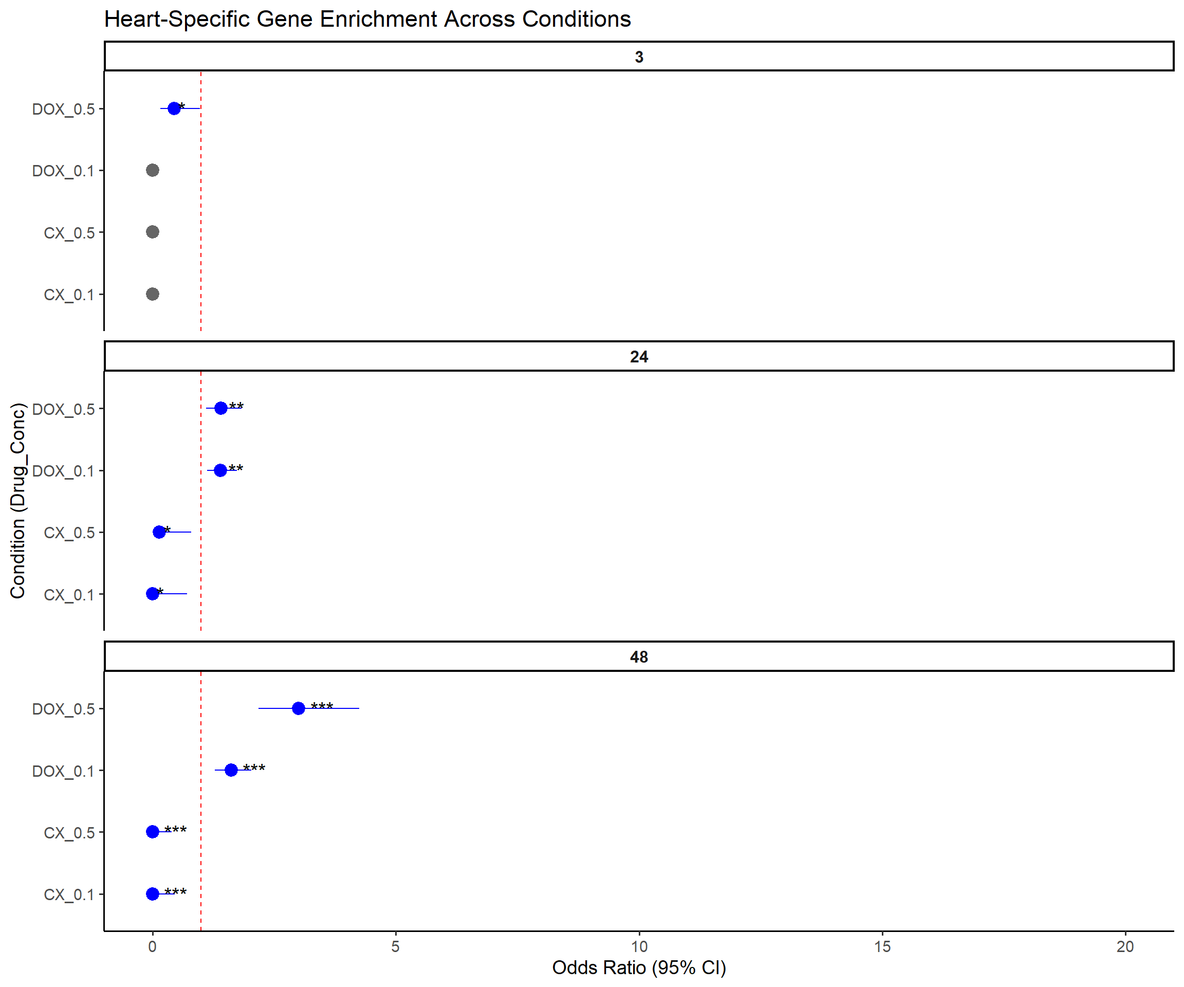
| Version | Author | Date |
|---|---|---|
| 64e2d5a | sayanpaul01 | 2025-10-06 |
# --- Step 7: Export results with raw counts ---
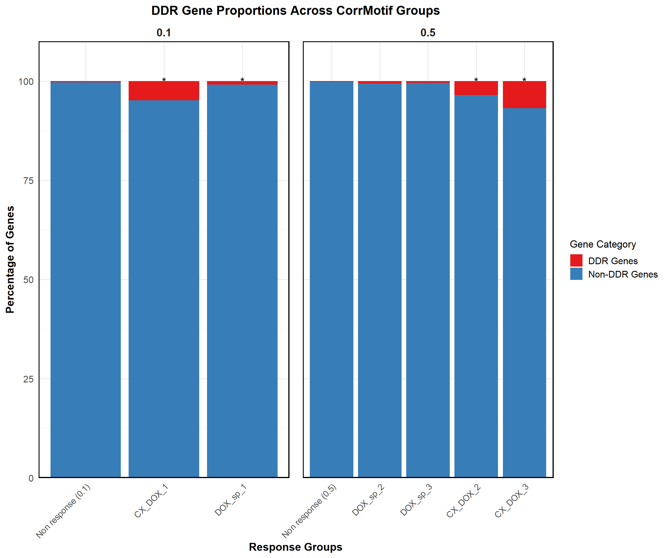
write.csv(results, "data/HeartSpecific_ForestPlot_Data.csv", row.names = FALSE)📌 Proportion of DDR Genes (CorrMotif Groups)
# ----------------- Load Required Libraries -----------------
library(dplyr)
library(ggplot2)

# ----------------- Load DDR Genes -----------------
ddr_entrez <- c(
  10111, 1017, 1019, 1020, 1021, 1026, 1027, 10912, 11011, 1111,
  11200, 1385, 1643, 1647, 1869, 207, 2177, 25, 27113, 27244,
  3014, 317, 355, 4193, 4292, 4361, 4609, 4616, 4683, 472, 50484,
  5366, 5371, 54205, 545, 55367, 5591, 581, 5810, 5883, 5884,
  5888, 5893, 5925, 595, 5981, 6118, 637, 672, 7157, 7799,
  8243, 836, 841, 84126, 842, 8795, 891, 894, 896, 898,
  9133, 9134, 983, 9874, 993, 995, 5916
) %>% as.character()

# ----------------- Load CorrMotif Groups -----------------
# 0.1 µM
prob_1_0.1 <- as.character(read.csv("data/prob_1_0.1.csv")$Entrez_ID)
prob_2_0.1 <- as.character(read.csv("data/prob_2_0.1.csv")$Entrez_ID)
prob_3_0.1 <- as.character(read.csv("data/prob_3_0.1.csv")$Entrez_ID)

# 0.5 µM
prob_1_0.5 <- as.character(read.csv("data/prob_1_0.5.csv")$Entrez_ID)
prob_2_0.5 <- as.character(read.csv("data/prob_2_0.5.csv")$Entrez_ID)
prob_3_0.5 <- as.character(read.csv("data/prob_3_0.5.csv")$Entrez_ID)
prob_4_0.5 <- as.character(read.csv("data/prob_4_0.5.csv")$Entrez_ID)
prob_5_0.5 <- as.character(read.csv("data/prob_5_0.5.csv")$Entrez_ID)

# ----------------- Annotate CorrMotif Groups -----------------
df_0.1 <- data.frame(Entrez_ID = unique(c(prob_1_0.1, prob_2_0.1, prob_3_0.1))) %>%
  mutate(
    Response_Group = case_when(
      Entrez_ID %in% prob_1_0.1 ~ "Non response (0.1)",
      Entrez_ID %in% prob_2_0.1 ~ "CX_DOX_1",
      Entrez_ID %in% prob_3_0.1 ~ "DOX_sp_1"
    ),
    Category = ifelse(Entrez_ID %in% ddr_entrez, "DDR Genes", "Non-DDR Genes"),
    Concentration = "0.1"
  )

df_0.5 <- data.frame(Entrez_ID = unique(c(prob_1_0.5, prob_2_0.5, prob_3_0.5, prob_4_0.5, prob_5_0.5))) %>%
  mutate(
    Response_Group = case_when(
      Entrez_ID %in% prob_1_0.5 ~ "Non response (0.5)",
      Entrez_ID %in% prob_2_0.5 ~ "DOX_sp_2",
      Entrez_ID %in% prob_3_0.5 ~ "DOX_sp_3",
      Entrez_ID %in% prob_4_0.5 ~ "CX_DOX_2",
      Entrez_ID %in% prob_5_0.5 ~ "CX_DOX_3"
    ),
    Category = ifelse(Entrez_ID %in% ddr_entrez, "DDR Genes", "Non-DDR Genes"),
    Concentration = "0.5"
  )

# ----------------- Combine Data -----------------
df_combined <- bind_rows(df_0.1, df_0.5)

# ----------------- Calculate Proportions -----------------
proportion_data <- df_combined %>%
  group_by(Concentration, Response_Group, Category) %>%
  summarise(Count = n(), .groups = "drop") %>%
  group_by(Concentration, Response_Group) %>%
  mutate(Percentage = Count / sum(Count) * 100)

# ----------------- Fisher's Exact Test -----------------
run_fisher_test <- function(df, ref_group) {
  ref_counts <- df %>%
    filter(Response_Group == ref_group) %>%
    dplyr::select(Category, Count) %>%
    {setNames(.$Count, .$Category)}

  df %>%
    filter(Response_Group != ref_group) %>%
    group_by(Response_Group) %>%
    summarise(
      p_value = {
        group_counts <- Count[Category %in% c("DDR Genes", "Non-DDR Genes")]
        if (length(group_counts) < 2) group_counts <- c(group_counts, 0)
        contingency_table <- matrix(c(
          group_counts[1], group_counts[2],
          ref_counts["DDR Genes"], ref_counts["Non-DDR Genes"]
        ), nrow = 2)
        fisher.test(contingency_table)$p.value
      },
      .groups = "drop"
    ) %>%
    mutate(Significance = ifelse(!is.na(p_value) & p_value < 0.05, "*", ""))
}

# Run Fisher’s test for each concentration
fisher_0.1 <- run_fisher_test(proportion_data %>% filter(Concentration == "0.1"), "Non response (0.1)")
fisher_0.5 <- run_fisher_test(proportion_data %>% filter(Concentration == "0.5"), "Non response (0.5)")

fisher_all <- bind_rows(
  fisher_0.1 %>% mutate(Concentration = "0.1"),
  fisher_0.5 %>% mutate(Concentration = "0.5")
)

# ----------------- Merge Fisher Results -----------------
proportion_data <- proportion_data %>%
  left_join(fisher_all, by = c("Concentration", "Response_Group"))

# ----------------- Reorder Groups -----------------
proportion_data$Response_Group <- factor(proportion_data$Response_Group, levels = c(
  "Non response (0.1)", "CX_DOX_1", "DOX_sp_1",
  "Non response (0.5)", "DOX_sp_2", "DOX_sp_3", "CX_DOX_2", "CX_DOX_3"
))

# ----------------- Star Labels -----------------
label_data <- proportion_data %>%
  group_by(Concentration, Response_Group) %>%
  summarise(Significance = dplyr::first(Significance), .groups = "drop") %>%
  filter(!is.na(Significance)) %>%
  mutate(y_pos = 100)

# ----------------- Plot -----------------
ggplot(proportion_data, aes(x = Response_Group, y = Percentage, fill = Category)) +
  geom_bar(stat = "identity", position = "stack") +
  geom_text(
    data = label_data,
    aes(x = Response_Group, y = y_pos, label = Significance),
    inherit.aes = FALSE,
    size = 5,
    color = "black"
  ) +
  facet_wrap(~ Concentration, scales = "free_x") +
  scale_fill_manual(values = c("DDR Genes" = "#e41a1c", "Non-DDR Genes" = "#377eb8")) +
  scale_y_continuous(limits = c(0, 110), expand = c(0, 0)) +
  labs(
    title = "DDR Gene Proportions Across CorrMotif Groups",
    x = "Response Groups",
    y = "Percentage of Genes",
    fill = "Gene Category"
  ) +
  theme_minimal(base_size = 14) +
  theme(
    plot.title = element_text(size = 16, hjust = 0.5, face = "bold"),
    axis.title.x = element_text(size = 14, face = "bold"),
    axis.title.y = element_text(size = 14, face = "bold"),
    axis.text.x = element_text(size = 11, angle = 45, hjust = 1),
    axis.text.y = element_text(size = 12),
    legend.title = element_text(size = 13),
    legend.text = element_text(size = 12),
    strip.text = element_text(size = 14, face = "bold"),
    panel.border = element_rect(color = "black", fill = NA, linewidth = 1.2),
    panel.spacing = unit(1.2, "lines")
  )
| Version | Author | Date |
|---|---|---|
| 64e2d5a | sayanpaul01 | 2025-10-06 |
📌 Odds Ratios for CorrMotif Groups (DDR genes)
library(dplyr)
library(tidyr)
library(tibble)
library(ggplot2)

# --- Load DDR Gene Entrez IDs ---
ddr_entrez <- c(
  10111, 1017, 1019, 1020, 1021, 1026, 1027, 10912, 11011, 1111,
  11200, 1385, 1643, 1647, 1869, 207, 2177, 25, 27113, 27244,
  3014, 317, 355, 4193, 4292, 4361, 4609, 4616, 4683, 472, 50484,
  5366, 5371, 54205, 545, 55367, 5591, 581, 5810, 5883, 5884,
  5888, 5893, 5925, 595, 5981, 6118, 637, 672, 7157, 7799,
  8243, 836, 841, 84126, 842, 8795, 891, 894, 896, 898,
  9133, 9134, 983, 9874, 993, 995, 5916
) %>% as.character()

# --- Load CorrMotif Groups ---
# 0.1 µM
prob_1_0.1 <- as.character(read.csv("data/prob_1_0.1.csv")$Entrez_ID)
prob_2_0.1 <- as.character(read.csv("data/prob_2_0.1.csv")$Entrez_ID)
prob_3_0.1 <- as.character(read.csv("data/prob_3_0.1.csv")$Entrez_ID)

# 0.5 µM
prob_1_0.5 <- as.character(read.csv("data/prob_1_0.5.csv")$Entrez_ID)
prob_2_0.5 <- as.character(read.csv("data/prob_2_0.5.csv")$Entrez_ID)
prob_3_0.5 <- as.character(read.csv("data/prob_3_0.5.csv")$Entrez_ID)
prob_4_0.5 <- as.character(read.csv("data/prob_4_0.5.csv")$Entrez_ID)
prob_5_0.5 <- as.character(read.csv("data/prob_5_0.5.csv")$Entrez_ID)

# --- Annotate Groups ---
df_0.1 <- data.frame(Entrez_ID = unique(c(prob_1_0.1, prob_2_0.1, prob_3_0.1))) %>%
  mutate(
    Response_Group = case_when(
      Entrez_ID %in% prob_1_0.1 ~ "Non response (0.1)",
      Entrez_ID %in% prob_2_0.1 ~ "CX_DOX_1",
      Entrez_ID %in% prob_3_0.1 ~ "DOX_sp_1"
    ),
    Category = ifelse(Entrez_ID %in% ddr_entrez, "DDR Genes", "Non-DDR Genes"),
    Concentration = "0.1"
  )

df_0.5 <- data.frame(Entrez_ID = unique(c(prob_1_0.5, prob_2_0.5, prob_3_0.5, prob_4_0.5, prob_5_0.5))) %>%
  mutate(
    Response_Group = case_when(
      Entrez_ID %in% prob_1_0.5 ~ "Non response (0.5)",
      Entrez_ID %in% prob_2_0.5 ~ "DOX_sp_2",
      Entrez_ID %in% prob_3_0.5 ~ "DOX_sp_3",
      Entrez_ID %in% prob_4_0.5 ~ "CX_DOX_2",
      Entrez_ID %in% prob_5_0.5 ~ "CX_DOX_3"
    ),
    Category = ifelse(Entrez_ID %in% ddr_entrez, "DDR Genes", "Non-DDR Genes"),
    Concentration = "0.5"
  )

df_combined <- bind_rows(df_0.1, df_0.5)

# --- Fisher Odds Ratio Function ---
fisher_or_group <- function(df_group, df_all, group_name, conc) {
  # counts in group
  a <- sum(df_group$Category == "DDR Genes")
  b <- sum(df_group$Category == "Non-DDR Genes")

  # counts in rest of groups at same conc
  ref <- df_all %>% filter(Response_Group != group_name)
  c <- sum(ref$Category == "DDR Genes")
  d <- sum(ref$Category == "Non-DDR Genes")

  mat <- matrix(c(a, b, c, d), nrow = 2)
  if (any(mat == 0)) mat <- mat + 0.5  # continuity correction

  test <- fisher.test(mat)

  tibble(
    Response_Group = group_name,
    Concentration  = conc,
    a = a, b = b, c = c, d = d,
    OR = unname(test$estimate),
    Lower_CI = test$conf.int[1],
    Upper_CI = test$conf.int[2],
    Pval = test$p.value,
    Stars = case_when(
      test$p.value < 0.001 ~ "***",
      test$p.value < 0.01  ~ "**",
      test$p.value < 0.05  ~ "*",
      TRUE ~ ""
    )
  )
}

# --- Run Fisher tests ---
results <- list()
for (conc in unique(df_combined$Concentration)) {
  conc_df <- df_combined %>% filter(Concentration == conc)
  for (grp in unique(conc_df$Response_Group)) {
    grp_df <- conc_df %>% filter(Response_Group == grp)
    results[[paste(conc, grp)]] <- fisher_or_group(grp_df, conc_df, grp, conc)
  }
}
results <- bind_rows(results)

# --- Save Results ---
write.csv(results, "data/CorrMotif_DDRGenes_OddsRatios.csv", row.names = FALSE)

# --- Forest Plot ---
ggplot(results, aes(x = Response_Group, y = OR, ymin = Lower_CI, ymax = Upper_CI)) +
  geom_pointrange(aes(color = Pval < 0.05), size = 0.9) +
  geom_text(aes(label = Stars), hjust = -0.5, size = 5) +
  geom_hline(yintercept = 1, linetype = "dashed", color = "red") +
  scale_color_manual(values = c("TRUE" = "blue", "FALSE" = "grey40")) +
  coord_flip() +
  facet_wrap(~Concentration, ncol = 1, scales = "free_y") +
  ylim(0, 20) +
  labs(
    title = "DDR Gene Enrichment Across CorrMotif Groups",
    x = "Response Group",
    y = "Odds Ratio (95% CI)"
  ) +
  theme_classic(base_size = 14) +
  theme(
    legend.position = "none",
    strip.text = element_text(face = "bold", size = 12)
  )
Warning: Removed 1 row containing missing values or values outside the scale range
(`geom_segment()`).Warning: Removed 2 rows containing missing values or values outside the scale range
(`geom_segment()`).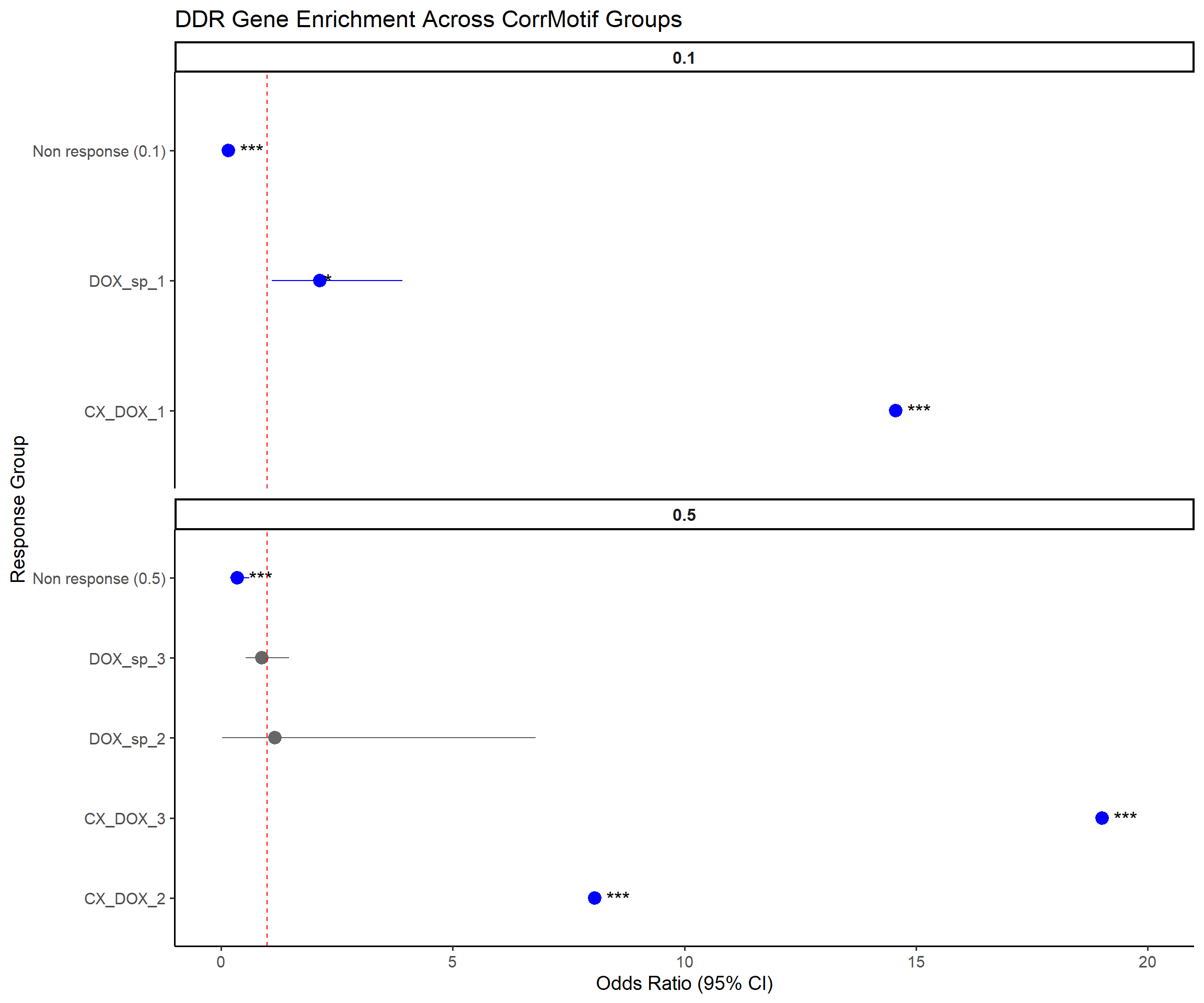
| Version | Author | Date |
|---|---|---|
| 64e2d5a | sayanpaul01 | 2025-10-06 |
📌 Violin-Boxplot: TS Score in 12 DEG samples
# 📦 Load Required Libraries
library(ggplot2)
library(dplyr)
library(tidyr)

# ✅ Step 1: Load DEG files
deg_list <- list(
  "CX_0.1_3"   = read.csv("data/DEGs/Toptable_CX_0.1_3.csv"),
  "CX_0.1_24"  = read.csv("data/DEGs/Toptable_CX_0.1_24.csv"),
  "CX_0.1_48"  = read.csv("data/DEGs/Toptable_CX_0.1_48.csv"),
  "CX_0.5_3"   = read.csv("data/DEGs/Toptable_CX_0.5_3.csv"),
  "CX_0.5_24"  = read.csv("data/DEGs/Toptable_CX_0.5_24.csv"),
  "CX_0.5_48"  = read.csv("data/DEGs/Toptable_CX_0.5_48.csv"),
  "DOX_0.1_3"  = read.csv("data/DEGs/Toptable_DOX_0.1_3.csv"),
  "DOX_0.1_24" = read.csv("data/DEGs/Toptable_DOX_0.1_24.csv"),
  "DOX_0.1_48" = read.csv("data/DEGs/Toptable_DOX_0.1_48.csv"),
  "DOX_0.5_3"  = read.csv("data/DEGs/Toptable_DOX_0.5_3.csv"),
  "DOX_0.5_24" = read.csv("data/DEGs/Toptable_DOX_0.5_24.csv"),
  "DOX_0.5_48" = read.csv("data/DEGs/Toptable_DOX_0.5_48.csv")
)

# ✅ Step 2: Load TS data
ts_data <- read.csv("data/TS.csv") %>%
  mutate(Entrez_ID = as.character(Entrez_ID))

# ✅ Step 3: Merge DEGs with TS scores
ts_long <- bind_rows(lapply(names(deg_list), function(name) {
  df <- deg_list[[name]] %>% filter(adj.P.Val < 0.05)
  df$Sample <- name
  df
})) %>%
  mutate(Entrez_ID = as.character(Entrez_ID)) %>%
  left_join(ts_data, by = "Entrez_ID") %>%
  separate(Sample, into = c("Drug","Conc","Time"), sep = "_") %>%
  mutate(
    Heart_Ventricle = as.numeric(Heart_Ventricle),
    Conc = factor(Conc, levels = c("0.1","0.5")),
    Time = factor(Time, levels = c("3","24","48"))   # ✅ enforce order
  ) %>%
  filter(!is.na(Heart_Ventricle))
Warning in left_join(., ts_data, by = "Entrez_ID"): Detected an unexpected many-to-many relationship between `x` and `y`.
ℹ Row 1904 of `x` matches multiple rows in `y`.
ℹ Row 6237 of `y` matches multiple rows in `x`.
ℹ If a many-to-many relationship is expected, set `relationship =
"many-to-many"` to silence this warning.Warning: There was 1 warning in `mutate()`.
ℹ In argument: `Heart_Ventricle = as.numeric(Heart_Ventricle)`.
Caused by warning:
! NAs introduced by coercion# ✅ Step 4: Define CX vs DOX comparison table
comparison_table <- expand.grid(
Conc = c("0.1","0.5"),
Time = c("3","24","48"),
stringsAsFactors = FALSE
)
# ✅ Step 5: Run Wilcoxon tests
star_df <- lapply(1:nrow(comparison_table), function(i) {
conc <- comparison_table$Conc[i]
time <- comparison_table$Time[i]
cx_vals <- ts_long$Heart_Ventricle[ts_long$Drug == "CX" & ts_long$Conc == conc & ts_long$Time == time]
dox_vals <- ts_long$Heart_Ventricle[ts_long$Drug == "DOX" & ts_long$Conc == conc & ts_long$Time == time]
cx_vals <- cx_vals[!is.na(cx_vals)]
dox_vals <- dox_vals[!is.na(dox_vals)]
if (length(cx_vals) > 2 & length(dox_vals) > 2) {
test_result <- wilcox.test(cx_vals, dox_vals)
pval <- test_result$p.value
if (pval < 0.05) {
label <- case_when(
pval < 0.001 ~ "***",
pval < 0.01 ~ "**",
TRUE ~ "*"
)
y_pos <- max(c(cx_vals, dox_vals), na.rm = TRUE) + 0.4
return(data.frame(
Conc = conc, Time = factor(time, levels = c("3","24","48")), # ✅ enforce order here too
label = label,
y_pos = y_pos
))
}
}
return(NULL)
}) %>% bind_rows()
# ✅ Step 6: Define colors
drug_colors <- c("CX" = "#1f78b4", "DOX" = "#e31a1c")
# ✅ Step 7: Violin + Boxplot
p <- ggplot(ts_long, aes(x = Drug, y = Heart_Ventricle, fill = Drug)) +
geom_violin(trim = FALSE, scale = "width", color = "black", alpha = 0.8) +
geom_boxplot(width = 0.2, color = "black", fill = "white", outlier.shape = NA) +
facet_grid(Conc ~ Time, scales = "free_x") +
scale_fill_manual(values = drug_colors) +
scale_y_continuous(
limits = c(-10, max(ts_long$Heart_Ventricle, na.rm = TRUE) + 2),
breaks = seq(-10, 25, 5)
) +
geom_hline(yintercept = 0, linetype = "dashed", color = "red") +
geom_text(
data = star_df,
aes(x = 1.5, y = y_pos, label = label),
inherit.aes = FALSE,
size = 6,
fontface = "bold"
) +
labs(
title = "Violin-Boxplot: Heart Ventricle TS (CX vs DOX DEGs)",
y = "Tissue specificity score (Heart Ventricle)",
x = ""
) +
theme_bw() +
theme(
axis.text.x = element_text(size = 12),
strip.text = element_text(size = 12, face = "bold"),
plot.title = element_text(size = 14, face = "bold", hjust = 0.5),
legend.position = "none"
)
print(p)Warning: Groups with fewer than two datapoints have been dropped.
ℹ Set `drop = FALSE` to consider such groups for position adjustment purposes.Warning: Computation failed in `stat_ydensity()`.
Caused by error in `$<-.data.frame`:
! replacement has 1 row, data has 0Warning: Groups with fewer than two datapoints have been dropped.
ℹ Set `drop = FALSE` to consider such groups for position adjustment purposes.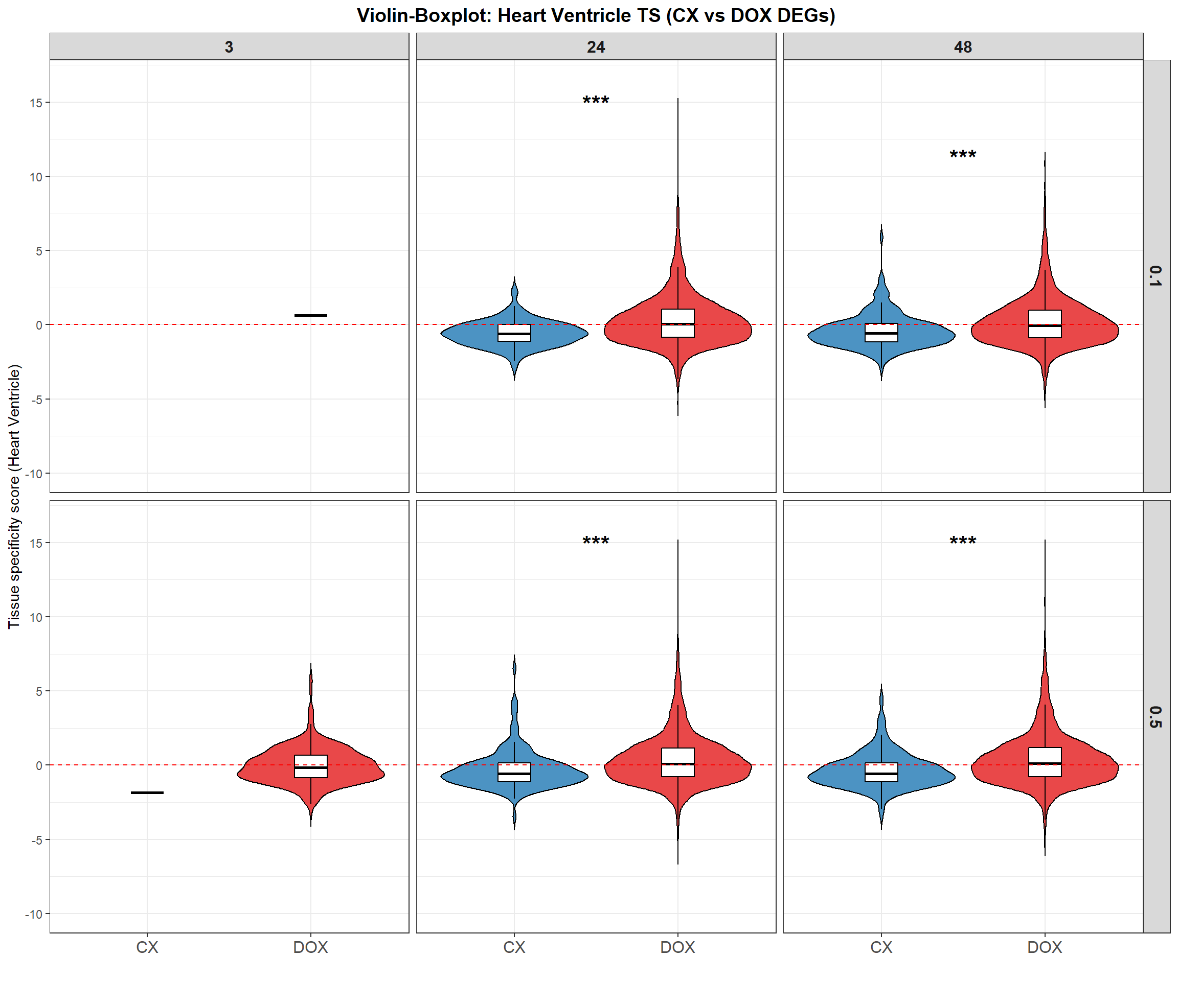
| Version | Author | Date |
|---|---|---|
| 64e2d5a | sayanpaul01 | 2025-10-06 |
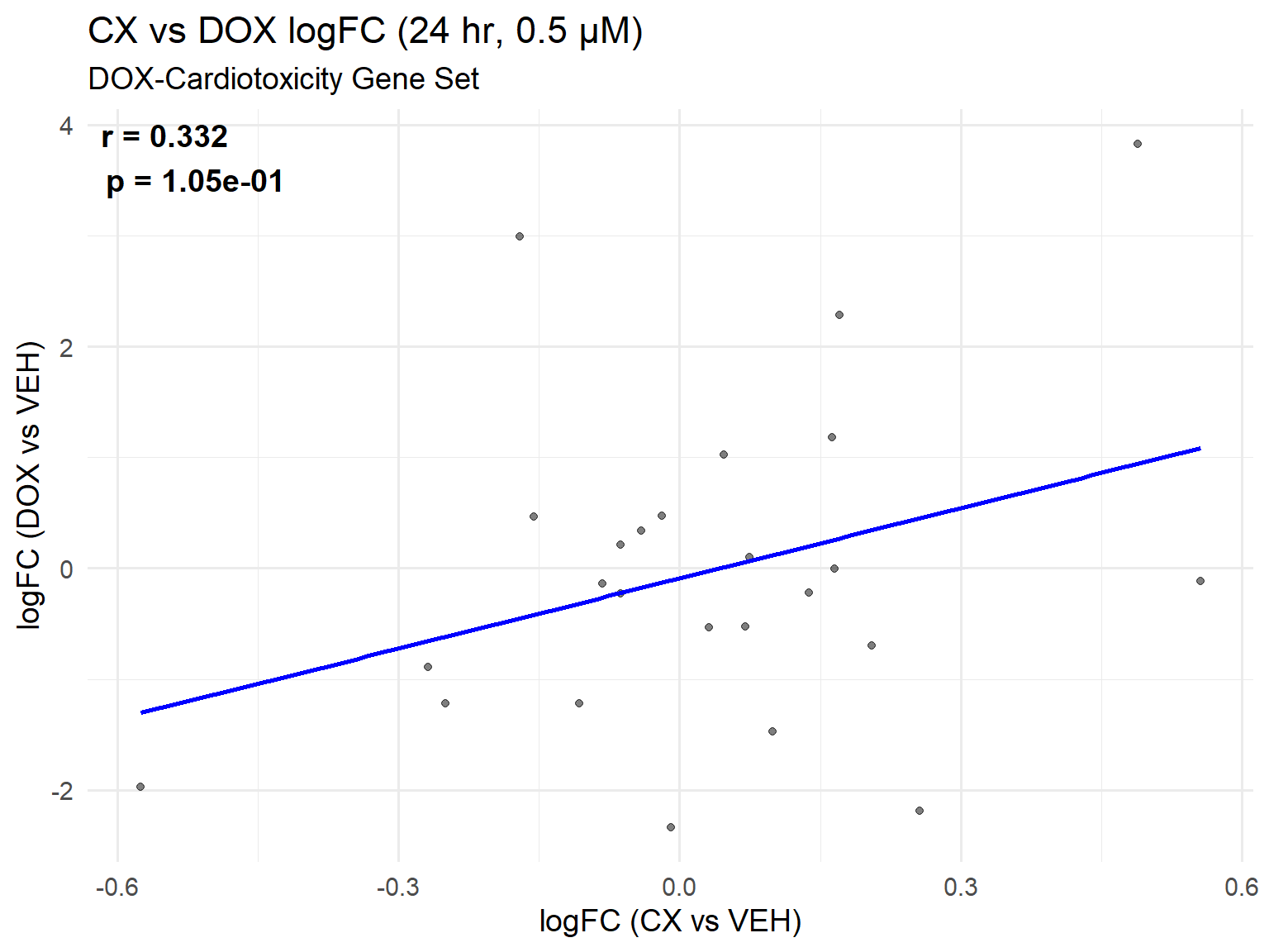
📌 DOX-Cardiotoxicity Gene Set Scatter Plot: CX vs DOX (0.5 µM, 24 hr)
library(ggplot2)

# --- Load Data ---
CX_0.5_24 <- read.csv("data/DEGs/Toptable_CX_0.5_24.csv")
DOX_0.5_24 <- read.csv("data/DEGs/Toptable_DOX_0.5_24.csv")

# --- Ensure Entrez_ID is character ---
CX_0.5_24$Entrez_ID <- as.character(CX_0.5_24$Entrez_ID)
DOX_0.5_24$Entrez_ID <- as.character(DOX_0.5_24$Entrez_ID)

# --- Merge on Entrez_ID ---
merged_24h_0.5 <- merge(
  CX_0.5_24, DOX_0.5_24,
  by = "Entrez_ID", suffixes = c("_CX", "_DOX")
)

# --- DOX-Cardiotoxicity Signature Entrez IDs ---
Entrez_IDs <- c(
  847, 873, 2064, 2878, 2944, 3038, 4846, 51196, 5880, 6687,
  7799, 4292, 5916, 3077, 51310, 9154, 64078, 5244, 10057, 10060,
  89845, 56853, 4625, 1573, 79890
)

# --- Subset merged data ---
cardio_set <- merged_24h_0.5[merged_24h_0.5$Entrez_ID %in% Entrez_IDs, ]

# --- Correlation ---
cor_test <- cor.test(
  cardio_set$logFC_CX,
  cardio_set$logFC_DOX,
  method = "pearson"
)

r_val <- round(cor_test$estimate, 3)
p_val <- formatC(cor_test$p.value, format = "e", digits = 2)
label_text <- paste0("r = ", r_val, "\n", "p = ", p_val)

# --- Scatter Plot (same style as 48 hr plot) ---
ggplot(cardio_set, aes(x = logFC_CX, y = logFC_DOX)) +
  geom_point(alpha = 0.5, color = "black") +
  geom_smooth(method = "lm", color = "blue", se = FALSE) +
  labs(
    title = "CX vs DOX logFC (24 hr, 0.5 µM)",
    subtitle = "DOX-Cardiotoxicity Gene Set",
    x = "logFC (CX vs VEH)",
    y = "logFC (DOX vs VEH)"
  ) +
  theme_minimal(base_size = 14) +
  annotate(
    "text",
    x = -Inf, y = Inf, hjust = -0.1, vjust = 1.2,
    label = label_text,
    size = 5, fontface = "bold"
  )
| Version | Author | Date |
|---|---|---|
| 64e2d5a | sayanpaul01 | 2025-10-06 |
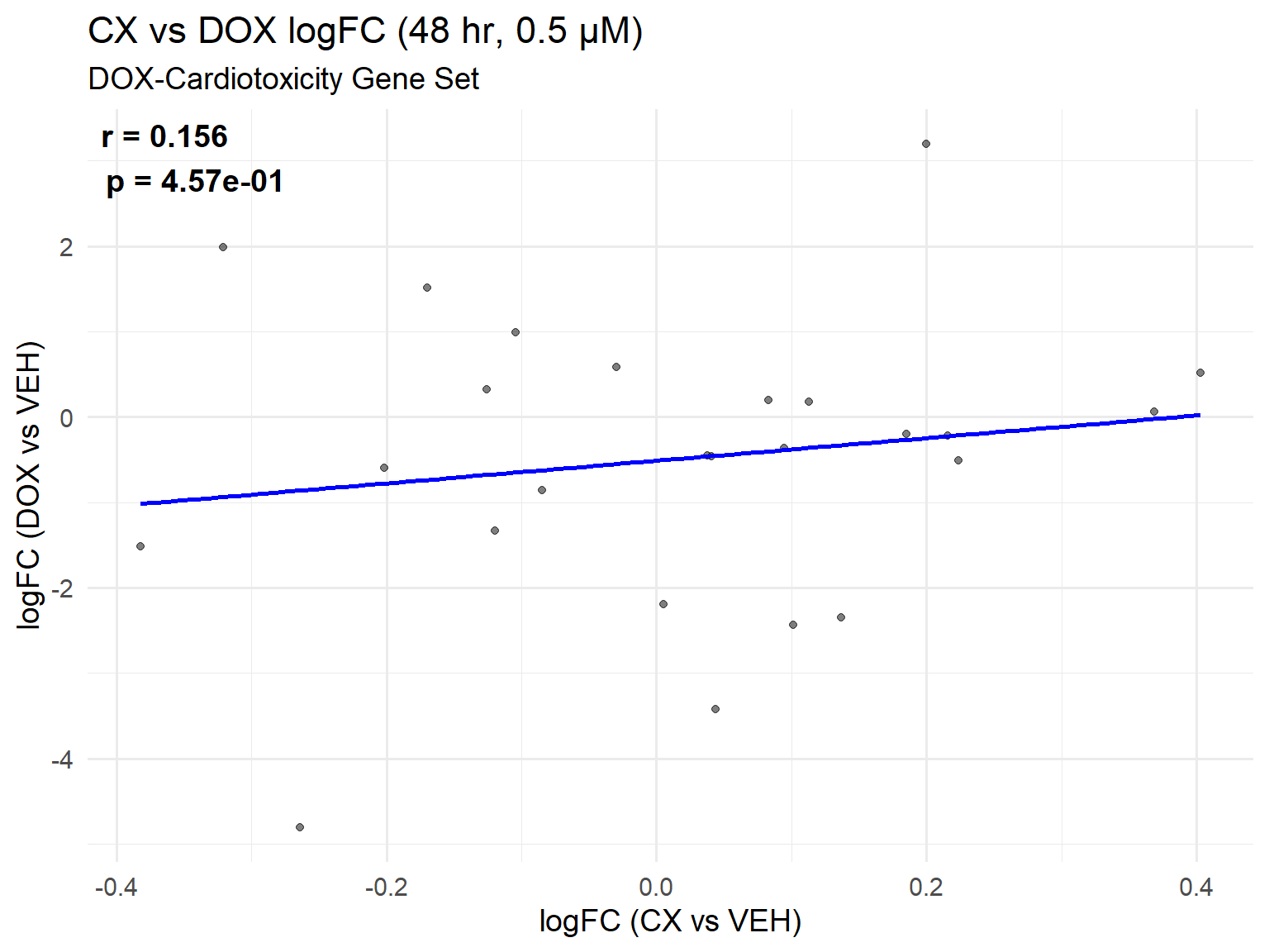
📌 DOX-Cardiotoxicity Gene Set Scatter Plot: CX vs DOX (0.5 µM, 48 hr)
library(ggplot2)

# --- Load Data ---
CX_0.5_48 <- read.csv("data/DEGs/Toptable_CX_0.5_48.csv")
DOX_0.5_48 <- read.csv("data/DEGs/Toptable_DOX_0.5_48.csv")

# --- Ensure Entrez_ID is character ---
CX_0.5_48$Entrez_ID <- as.character(CX_0.5_48$Entrez_ID)
DOX_0.5_48$Entrez_ID <- as.character(DOX_0.5_48$Entrez_ID)

# --- Merge on Entrez_ID ---
merged_48h_0.5 <- merge(
  CX_0.5_48, DOX_0.5_48,
  by = "Entrez_ID", suffixes = c("_CX", "_DOX")
)

# --- DOX-Cardiotoxicity Signature Entrez IDs ---
Entrez_IDs <- c(
  847, 873, 2064, 2878, 2944, 3038, 4846, 51196, 5880, 6687,
  7799, 4292, 5916, 3077, 51310, 9154, 64078, 5244, 10057, 10060,
  89845, 56853, 4625, 1573, 79890
)

# --- Subset merged data ---
cardio_set_48 <- merged_48h_0.5[merged_48h_0.5$Entrez_ID %in% Entrez_IDs, ]

# --- Correlation ---
cor_test <- cor.test(
  cardio_set_48$logFC_CX,
  cardio_set_48$logFC_DOX,
  method = "pearson"
)

r_val <- round(cor_test$estimate, 3)
p_val <- formatC(cor_test$p.value, format = "e", digits = 2)
label_text <- paste0("r = ", r_val, "\n", "p = ", p_val)

# --- Scatter Plot (same publication style) ---
ggplot(cardio_set_48, aes(x = logFC_CX, y = logFC_DOX)) +
  geom_point(alpha = 0.5, color = "black") +
  geom_smooth(method = "lm", color = "blue", se = FALSE) +
  labs(
    title = "CX vs DOX logFC (48 hr, 0.5 µM)",
    subtitle = "DOX-Cardiotoxicity Gene Set",
    x = "logFC (CX vs VEH)",
    y = "logFC (DOX vs VEH)"
  ) +
  theme_minimal(base_size = 14) +
  annotate(
    "text",
    x = -Inf, y = Inf, hjust = -0.1, vjust = 1.2,
    label = label_text,
    size = 5, fontface = "bold"
  )
| Version | Author | Date |
|---|---|---|
| 64e2d5a | sayanpaul01 | 2025-10-06 |
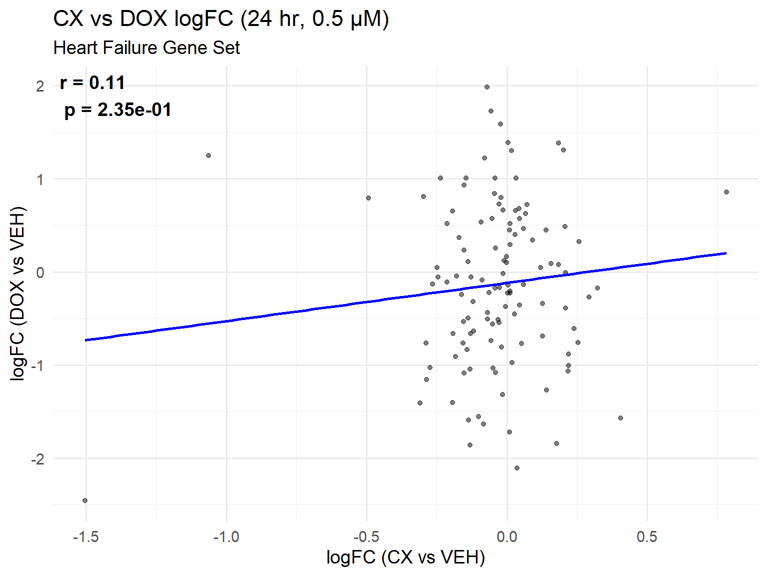
📌 Heart Failure Gene Set Scatter Plot: CX vs DOX (0.5 µM, 24 hr)
library(ggplot2)
library(dplyr)

# --- Load Data ---
CX_0.5_24 <- read.csv("data/DEGs/Toptable_CX_0.5_24.csv")
DOX_0.5_24 <- read.csv("data/DEGs/Toptable_DOX_0.5_24.csv")

# --- Ensure Entrez_ID is character ---
CX_0.5_24$Entrez_ID <- as.character(CX_0.5_24$Entrez_ID)
DOX_0.5_24$Entrez_ID <- as.character(DOX_0.5_24$Entrez_ID)

# --- Merge on Entrez_ID ---
merged_24h_0.5 <- merge(
  CX_0.5_24, DOX_0.5_24,
  by = "Entrez_ID", suffixes = c("_CX", "_DOX")
)

# --- Heart Failure Gene Set ---
entrez_ids <- c(
  9709, 8882, 4023, 29959, 5496, 3992, 9415, 5308, 1026, 54437, 79068, 10221,
  9031, 1187, 1952, 3705, 84722, 7273, 23293, 155382, 9531, 602, 27258, 84163,
  81846, 79933, 56911, 64753, 93210, 1021, 283450, 5998, 57602, 114991, 7073,
  3156, 100101267, 22996, 285025, 11080, 11124, 54810, 7531, 27241, 4774, 57794,
  463, 91319, 6598, 9640, 2186, 26010, 80816, 571, 88, 51652, 64788, 90523, 2969,
  7781, 80777, 10725, 23387, 817, 134728, 8842, 949, 6934, 129787, 10327, 202052,
  2318, 5578, 6801, 6311, 10019, 80724, 217, 84909, 388591, 55101, 9839, 27161,
  5310, 387119, 4641, 5587, 55188, 222553, 9960, 22852, 10087, 9570, 54497,
  200942, 26249, 4137, 375056, 5409, 64116, 8291, 22876, 339855, 4864, 5142,
  221692, 55023, 51426, 6146, 84251, 8189, 27332, 57099, 1869, 1112, 23327,
  11264, 6001
) %>% as.character()

# --- Subset merged data ---
heart_set <- merged_24h_0.5[merged_24h_0.5$Entrez_ID %in% entrez_ids, ]

# --- Correlation ---
cor_test <- cor.test(
  heart_set$logFC_CX,
  heart_set$logFC_DOX,
  method = "pearson"
)

r_val <- round(cor_test$estimate, 3)
p_val <- formatC(cor_test$p.value, format = "e", digits = 2)
label_text <- paste0("r = ", r_val, "\n", "p = ", p_val)

# --- Scatter Plot (same style) ---
ggplot(heart_set, aes(x = logFC_CX, y = logFC_DOX)) +
  geom_point(alpha = 0.5, color = "black") +
  geom_smooth(method = "lm", color = "blue", se = FALSE) +
  labs(
    title = "CX vs DOX logFC (24 hr, 0.5 µM)",
    subtitle = "Heart Failure Gene Set",
    x = "logFC (CX vs VEH)",
    y = "logFC (DOX vs VEH)"
  ) +
  theme_minimal(base_size = 14) +
  annotate(
    "text",
    x = -Inf, y = Inf,
    hjust = -0.1, vjust = 1.2,
    label = label_text,
    size = 5, fontface = "bold"
  )
| Version | Author | Date |
|---|---|---|
| 64e2d5a | sayanpaul01 | 2025-10-06 |
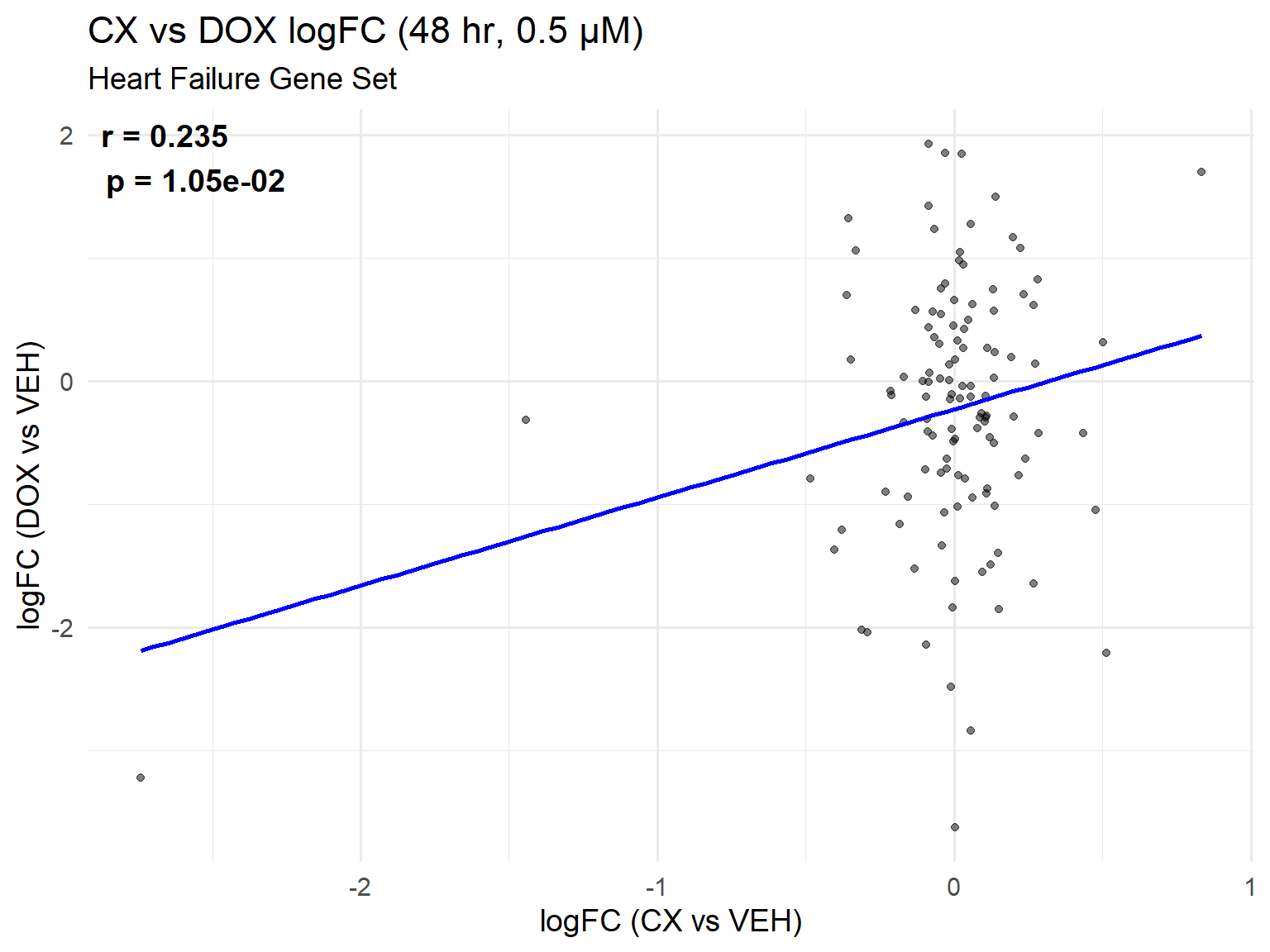
📌 Heart Failure Gene Set Scatter Plot: CX vs DOX (0.5 µM, 48 hr)
library(ggplot2)
library(dplyr)

# --- Load Data ---
CX_0.5_48 <- read.csv("data/DEGs/Toptable_CX_0.5_48.csv")
DOX_0.5_48 <- read.csv("data/DEGs/Toptable_DOX_0.5_48.csv")

# --- Ensure Entrez_ID is character ---
CX_0.5_48$Entrez_ID <- as.character(CX_0.5_48$Entrez_ID)
DOX_0.5_48$Entrez_ID <- as.character(DOX_0.5_48$Entrez_ID)

# --- Merge on Entrez_ID ---
merged_48h_0.5 <- merge(
  CX_0.5_48, DOX_0.5_48,
  by = "Entrez_ID", suffixes = c("_CX", "_DOX")
)

# --- Heart Failure Gene Set ---
entrez_ids <- c(
  9709, 8882, 4023, 29959, 5496, 3992, 9415, 5308, 1026, 54437, 79068, 10221,
  9031, 1187, 1952, 3705, 84722, 7273, 23293, 155382, 9531, 602, 27258, 84163,
  81846, 79933, 56911, 64753, 93210, 1021, 283450, 5998, 57602, 114991, 7073,
  3156, 100101267, 22996, 285025, 11080, 11124, 54810, 7531, 27241, 4774, 57794,
  463, 91319, 6598, 9640, 2186, 26010, 80816, 571, 88, 51652, 64788, 90523, 2969,
  7781, 80777, 10725, 23387, 817, 134728, 8842, 949, 6934, 129787, 10327, 202052,
  2318, 5578, 6801, 6311, 10019, 80724, 217, 84909, 388591, 55101, 9839, 27161,
  5310, 387119, 4641, 5587, 55188, 222553, 9960, 22852, 10087, 9570, 54497,
  200942, 26249, 4137, 375056, 5409, 64116, 8291, 22876, 339855, 4864, 5142,
  221692, 55023, 51426, 6146, 84251, 8189, 27332, 57099, 1869, 1112, 23327,
  11264, 6001
) %>% as.character()

# --- Subset merged data ---
heart_set_48 <- merged_48h_0.5[merged_48h_0.5$Entrez_ID %in% entrez_ids, ]

# --- Correlation ---
cor_test <- cor.test(
  heart_set_48$logFC_CX,
  heart_set_48$logFC_DOX,
  method = "pearson"
)

r_val <- round(cor_test$estimate, 3)
p_val <- formatC(cor_test$p.value, format = "e", digits = 2)
label_text <- paste0("r = ", r_val, "\n", "p = ", p_val)

# --- Scatter Plot (matching style) ---
ggplot(heart_set_48, aes(x = logFC_CX, y = logFC_DOX)) +
  geom_point(alpha = 0.5, color = "black") +
  geom_smooth(method = "lm", color = "blue", se = FALSE) +
  labs(
    title = "CX vs DOX logFC (48 hr, 0.5 µM)",
    subtitle = "Heart Failure Gene Set",
    x = "logFC (CX vs VEH)",
    y = "logFC (DOX vs VEH)"
  ) +
  theme_minimal(base_size = 14) +
  annotate(
    "text",
    x = -Inf, y = Inf,
    hjust = -0.1, vjust = 1.2,
    label = label_text,
    size = 5, fontface = "bold"
  )
| Version | Author | Date |
|---|---|---|
| 64e2d5a | sayanpaul01 | 2025-10-06 |
📌 Forest Plot: Atrial Fibrillation (AF) Risk Loci Enrichment
# --- Libraries ---
library(dplyr)
library(tidyr)
library(tibble)
library(ggplot2)
library(readr)

# --- Step 1: Load AF Risk Loci (Entrez IDs) ---
# Option 1: If you saved it earlier
# entrez_ids <- readRDS("data/AF_Entrez_IDs.rds")

# Option 2: Or load from mapped CSV (ensure column name is Entrez_ID)
AF_genes <- read.csv("data/Cleaned_AF_genes_with_Entrez.csv", stringsAsFactors = FALSE)
entrez_ids <- AF_genes$Entrez_ID %>% as.character() %>% unique() %>% na.omit()

cat("✅ Loaded", length(entrez_ids), "AF Entrez IDs.\n")
✅ Loaded 615 AF Entrez IDs.# --- Step 2: Load DEG tables ---
deg_files <- list.files("data/DEGs/", pattern = "Toptable_.*\\.csv", full.names = TRUE)
if (length(deg_files) == 0) stop("❌ No DEG files found in data/DEGs/")
deg_list <- lapply(deg_files, read.csv)
names(deg_list) <- gsub("Toptable_|\\.csv", "", basename(deg_files))
# --- Step 3: Fisher test function ---
fisher_or <- function(df, sample_name) {
if (!"Entrez_ID" %in% colnames(df)) return(NULL)
df <- df %>%
mutate(
DEG = adj.P.Val < 0.05,
AF_risk = Entrez_ID %in% entrez_ids
)
a <- sum(df$DEG & df$AF_risk, na.rm = TRUE)
b <- sum(df$DEG & !df$AF_risk, na.rm = TRUE)
c <- sum(!df$DEG & df$AF_risk, na.rm = TRUE)
d <- sum(!df$DEG & !df$AF_risk, na.rm = TRUE)
# Fisher’s exact test
test <- tryCatch(
fisher.test(matrix(c(a, b, c, d), nrow = 2)),
error = function(e) fisher.test(matrix(c(a, b, c, d), nrow = 2), simulate.p.value = TRUE)
)
tibble(
Sample = sample_name,
DE_Risk = a,
DE_nonRisk = b,
nonDE_Risk = c,
nonDE_nonRisk = d,
OR = unname(test$estimate),
Lower_CI = test$conf.int[1],
Upper_CI = test$conf.int[2],
Pval = test$p.value,
Stars = case_when(
test$p.value < 0.001 ~ "***",
test$p.value < 0.01 ~ "**",
test$p.value < 0.05 ~ "*",
TRUE ~ ""
)
)
}
# --- Step 4: Run Fisher tests for all DEG tables ---
results <- bind_rows(mapply(fisher_or, deg_list, names(deg_list), SIMPLIFY = FALSE))
# --- Step 5: Extract metadata (Drug, Conc, Time) ---
results <- results %>%
separate(Sample, into = c("Drug","Conc","Time"), sep = "_") %>%
mutate(
Label = paste(Drug, Conc, sep = "_"),
Time = factor(Time, levels = c("3","24","48"))
)
# --- Step 6: Forest plot ---
p <- ggplot(results, aes(x = Label, y = OR, ymin = Lower_CI, ymax = Upper_CI)) +
geom_pointrange(aes(color = Pval < 0.05), size = 0.9) +
geom_text(aes(label = Stars), hjust = -0.5, size = 5) +
geom_hline(yintercept = 1, linetype = "dashed", color = "red") +
scale_color_manual(values = c("TRUE" = "blue", "FALSE" = "grey40")) +
coord_flip() +
facet_wrap(~Time, ncol = 1, scales = "free_y") +
ylim(0, 20) +
labs(
title = "Atrial Fibrillation Risk Loci Enrichment Across Conditions",
x = "Condition (Drug_Conc)",
y = "Odds Ratio (95% CI)"
) +
theme_classic(base_size = 14) +
theme(
legend.position = "none",
strip.text = element_text(face = "bold", size = 12)
)
# --- Step 7: Display & save ---
print(p)Warning: Removed 3 rows containing missing values or values outside the scale range
(`geom_segment()`).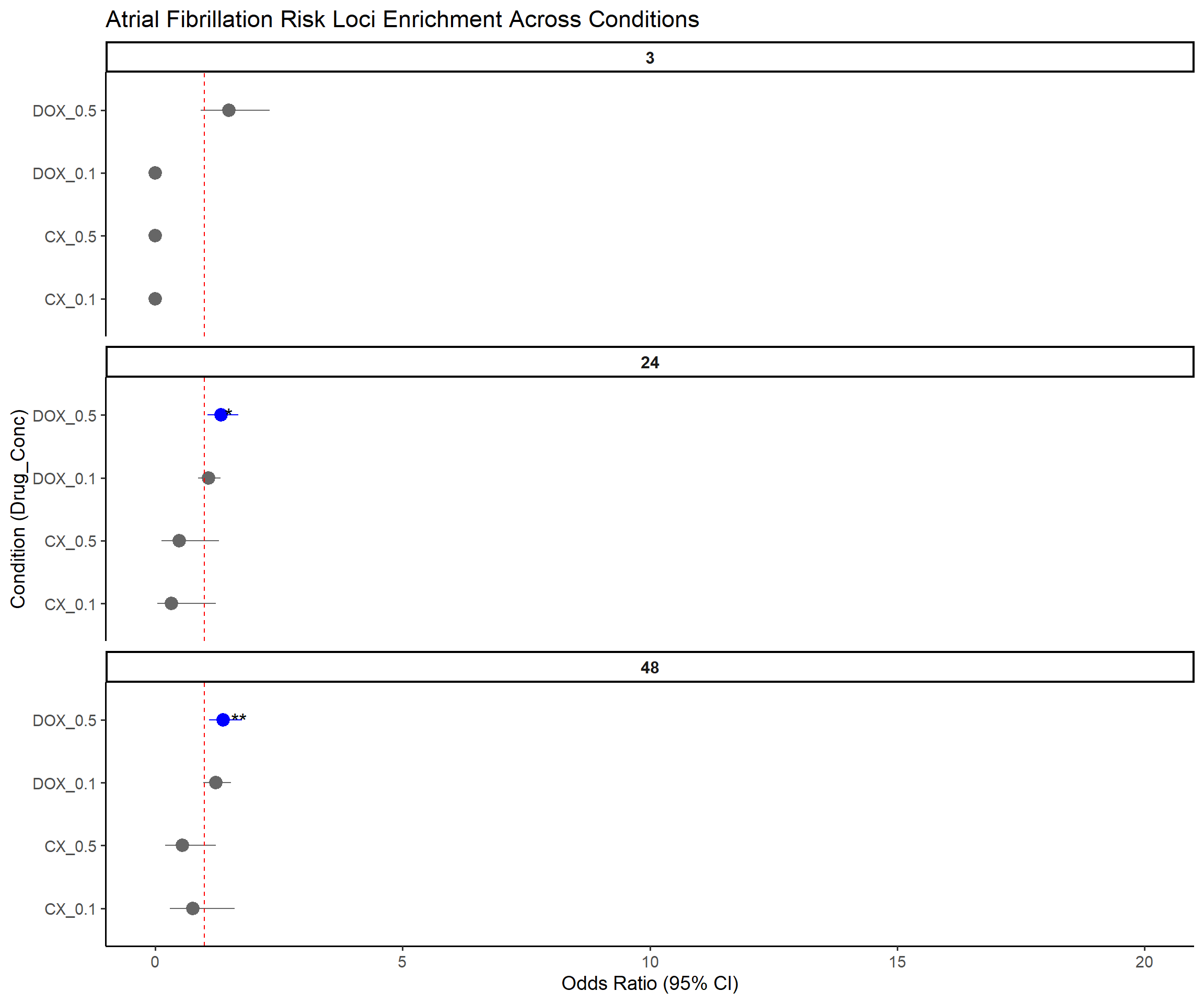
| Version | Author | Date |
|---|---|---|
| 64e2d5a | sayanpaul01 | 2025-10-06 |
#ggsave("plots/ForestPlot_AF_RiskLoci.png", plot = p, width = 7, height = 9, dpi = 300)

# --- Step 8: Export raw enrichment data ---
write.csv(results, "data/AF_Cardiotoxicity_ForestPlot_Data.csv", row.names = FALSE)

cat("✅ AF enrichment analysis complete. Results saved to data/AF_Cardiotoxicity_ForestPlot_Data.csv\n")
✅ AF enrichment analysis complete. Results saved to data/AF_Cardiotoxicity_ForestPlot_Data.csv📌 Odds Ratios for CorrMotif Groups (AF genes)
library(dplyr)
library(tidyr)
library(tibble)
library(ggplot2)

# --- Load AF Gene Entrez IDs ---
# Option 1: from mapped CSV
AF_genes <- read.csv("data/Cleaned_AF_genes_with_Entrez.csv", stringsAsFactors = FALSE)
af_entrez <- AF_genes$Entrez_ID %>% as.character() %>% unique() %>% na.omit()

# Option 2: if saved as RDS earlier
# af_entrez <- readRDS("data/AF_Entrez_IDs.rds")

cat("✅ Loaded", length(af_entrez), "AF Entrez IDs.\n")
✅ Loaded 615 AF Entrez IDs.# --- Load CorrMotif Groups ---
# 0.1 µM
prob_1_0.1 <- as.character(read.csv("data/prob_1_0.1.csv")$Entrez_ID)
prob_2_0.1 <- as.character(read.csv("data/prob_2_0.1.csv")$Entrez_ID)
prob_3_0.1 <- as.character(read.csv("data/prob_3_0.1.csv")$Entrez_ID)
# 0.5 µM
prob_1_0.5 <- as.character(read.csv("data/prob_1_0.5.csv")$Entrez_ID)
prob_2_0.5 <- as.character(read.csv("data/prob_2_0.5.csv")$Entrez_ID)
prob_3_0.5 <- as.character(read.csv("data/prob_3_0.5.csv")$Entrez_ID)
prob_4_0.5 <- as.character(read.csv("data/prob_4_0.5.csv")$Entrez_ID)
prob_5_0.5 <- as.character(read.csv("data/prob_5_0.5.csv")$Entrez_ID)
# --- Annotate Groups ---
df_0.1 <- data.frame(Entrez_ID = unique(c(prob_1_0.1, prob_2_0.1, prob_3_0.1))) %>%
mutate(
Response_Group = case_when(
Entrez_ID %in% prob_1_0.1 ~ "Non response (0.1)",
Entrez_ID %in% prob_2_0.1 ~ "CX_DOX_1",
Entrez_ID %in% prob_3_0.1 ~ "DOX_sp_1"
),
Category = ifelse(Entrez_ID %in% af_entrez, "AF Genes", "Non-AF Genes"),
Concentration = "0.1"
)
df_0.5 <- data.frame(Entrez_ID = unique(c(prob_1_0.5, prob_2_0.5, prob_3_0.5, prob_4_0.5, prob_5_0.5))) %>%
mutate(
Response_Group = case_when(
Entrez_ID %in% prob_1_0.5 ~ "Non response (0.5)",
Entrez_ID %in% prob_2_0.5 ~ "DOX_sp_2",
Entrez_ID %in% prob_3_0.5 ~ "DOX_sp_3",
Entrez_ID %in% prob_4_0.5 ~ "CX_DOX_2",
Entrez_ID %in% prob_5_0.5 ~ "CX_DOX_3"
),
Category = ifelse(Entrez_ID %in% af_entrez, "AF Genes", "Non-AF Genes"),
Concentration = "0.5"
)
# --- Combine all CorrMotif groups ---
df_combined <- bind_rows(df_0.1, df_0.5)
# --- Fisher Odds Ratio Function ---
fisher_or_group <- function(df_group, df_all, group_name, conc) {
# counts in group
a <- sum(df_group$Category == "AF Genes")
b <- sum(df_group$Category == "Non-AF Genes")
# counts in rest of groups at same concentration
ref <- df_all %>% filter(Response_Group != group_name)
c <- sum(ref$Category == "AF Genes")
d <- sum(ref$Category == "Non-AF Genes")
mat <- matrix(c(a, b, c, d), nrow = 2)
if (any(mat == 0)) mat <- mat + 0.5 # continuity correction
test <- fisher.test(mat)
tibble(
Response_Group = group_name,
Concentration = conc,
a = a, b = b, c = c, d = d,
OR = unname(test$estimate),
Lower_CI = test$conf.int[1],
Upper_CI = test$conf.int[2],
Pval = test$p.value,
Stars = case_when(
test$p.value < 0.001 ~ "***",
test$p.value < 0.01 ~ "**",
test$p.value < 0.05 ~ "*",
TRUE ~ ""
)
)
}
# --- Run Fisher tests across groups ---
results <- list()
for (conc in unique(df_combined$Concentration)) {
conc_df <- df_combined %>% filter(Concentration == conc)
for (grp in unique(conc_df$Response_Group)) {
grp_df <- conc_df %>% filter(Response_Group == grp)
results[[paste(conc, grp)]] <- fisher_or_group(grp_df, conc_df, grp, conc)
}
}
results <- bind_rows(results)
# --- Save Results ---
write.csv(results, "data/CorrMotif_AFGenes_OddsRatios.csv", row.names = FALSE)
cat("✅ Results saved to data/CorrMotif_AFGenes_OddsRatios.csv\n")✅ Results saved to data/CorrMotif_AFGenes_OddsRatios.csv# --- Forest Plot ---
p <- ggplot(results, aes(x = Response_Group, y = OR, ymin = Lower_CI, ymax = Upper_CI)) +
geom_pointrange(aes(color = Pval < 0.05), size = 0.9) +
geom_text(aes(label = Stars), hjust = -0.5, size = 5) +
geom_hline(yintercept = 1, linetype = "dashed", color = "red") +
scale_color_manual(values = c("TRUE" = "blue", "FALSE" = "grey40")) +
coord_flip() +
facet_wrap(~Concentration, ncol = 1, scales = "free_y") +
ylim(0, 20) +
labs(
title = "AF Gene Enrichment Across CorrMotif Groups",
x = "Response Group",
y = "Odds Ratio (95% CI)"
) +
theme_classic(base_size = 14) +
theme(
legend.position = "none",
strip.text = element_text(face = "bold", size = 12)
)
p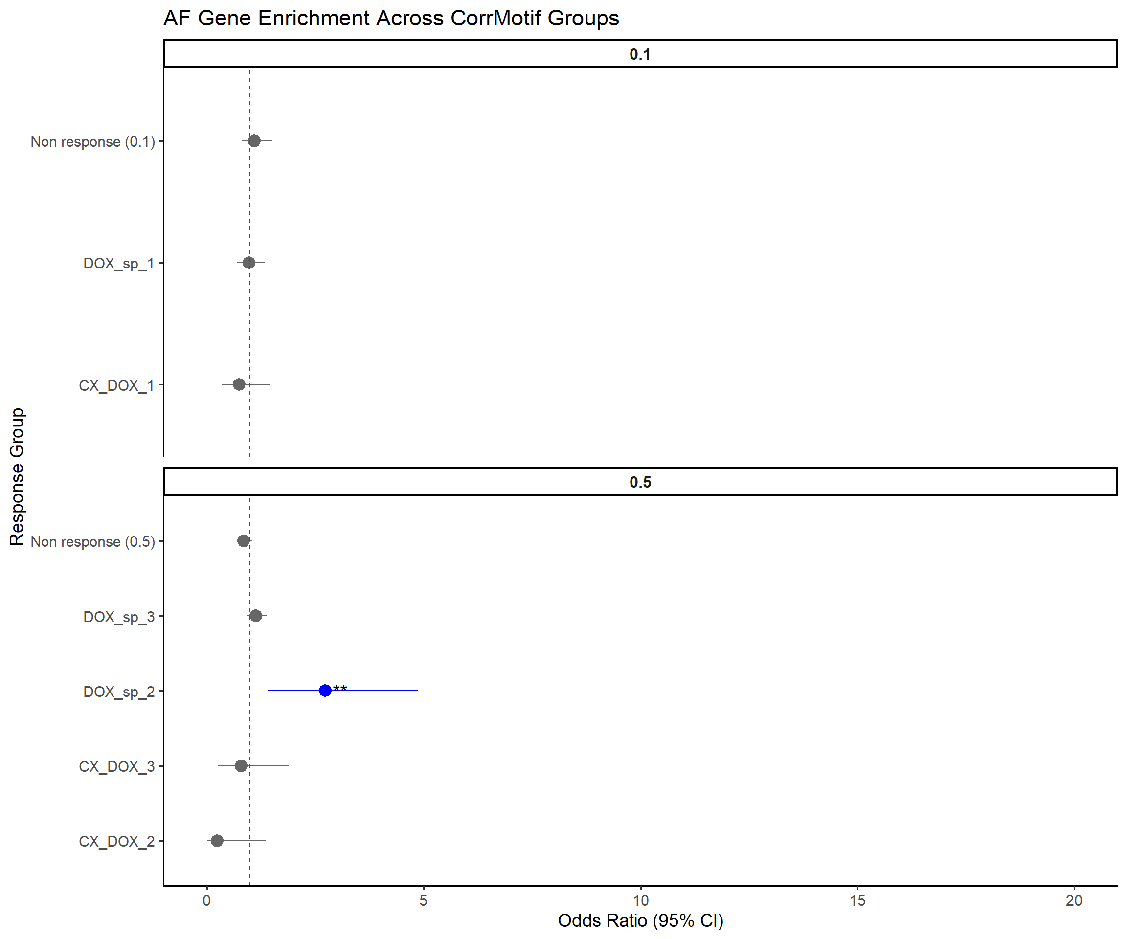
| Version | Author | Date |
|---|---|---|
| 64e2d5a | sayanpaul01 | 2025-10-06 |
📌CX-5461 Sensitivity Comparison (All values in µM) Unified naming: LD50 (µM)
library(ggplot2)
library(dplyr)

## === iPSC-CM LD50 (µM) ===
ipsc_vals <- c(6.4, 10.9, 10.0)
ipsc_df <- data.frame(
  CellLine = c("iPSC-CM_1", "iPSC-CM_2", "iPSC-CM_3"),
  LD50 = ipsc_vals,
  Group = "iPSC-CM"
)

## === Sanij et al. (GI50 nM → µM, renamed as LD50) ===
sanij_data <- data.frame(
  CellLine = c("OVCAR3","FUOV1","COLO704","TOV112D","CH1","A2780","RMGI","2008","SKOV3","OVCA432",
               "OAW42","ES2","EFO27","IGROV1","Caov3","Colo720E","MCAS","OVCAR5","OVCAR4","OVCAR8",
               "JHOC5","JHOM1","KURAMOCHI","JHOC7","JHOS3","RMGII","OAW28","OV90"),
  Mean_nM = c(12,25.33,31.5,49.67,73.5,82.33,143,106.7,301.3,206.7,
              226.7,181.3,417,422.3,409.3,413.5,357.6,100.5,613.3,859,
              731,861.2,1082,3267,3177,3370,3850,5170)
) %>%
  dplyr::mutate(
    LD50 = Mean_nM / 1000,  # convert to µM
    Group = ifelse(Mean_nM < 2000, "Sensitive", "Resistant")
  ) %>%
  dplyr::select(CellLine, LD50, Group)

## === Cornelison et al. (IC50 µM, renamed as LD50) ===
cornelison <- data.frame(
  CellLine = c("A2780ip2","A2780cp20","SKOV3ip1","SKOV3TRip2",
               "HeyA8","HeyA8MDR","PEO1","PEO4","OV90","OVCAR3",
               "OAW42","OVSAHO","CAOV3","COV362","ES2","HIO-180"),
  LD50 = c(0.032,0.146,0.595,0.109,
           2.05,0.191,0.525,1.20,1.06,2.00,
           0.300,0.636,0.955,0.645,0.294,5.49),
  Group = c(rep("Sensitive",15),"Resistant")
)

## === Combine all datasets ===
all_data <- dplyr::bind_rows(sanij_data, cornelison, ipsc_df)

## === Plot (linear scale) ===
ggplot(all_data, aes(x = Group, y = LD50, fill = Group)) +
  geom_boxplot(outlier.shape = NA, alpha = 0.6, width = 0.6,
               color = "black", linewidth = 0.4) +
  geom_point(aes(color = Group),
             position = position_nudge(x = 0),
             size = 3, alpha = 0.9, show.legend = FALSE) +
  scale_fill_manual(values = c("Sensitive"="#4A90E2",
                               "Resistant"="#B0B0B0",
                               "iPSC-CM"="#E74C3C")) +
  scale_color_manual(values = c("Sensitive"="#4A90E2",
                                "Resistant"="#B0B0B0",
                                "iPSC-CM"="#E74C3C")) +
  labs(
    title = expression("CX-5461 Sensitivity (LD"[50]*", µM)"),
    x = "",
    y = expression("LD"[50]*" (µM)")
  ) +
  theme_minimal(base_size = 14) +
  theme(
    legend.position = "right",
    plot.title = element_text(hjust = 0.5, face = "bold"),
    axis.text = element_text(color = "black")
  )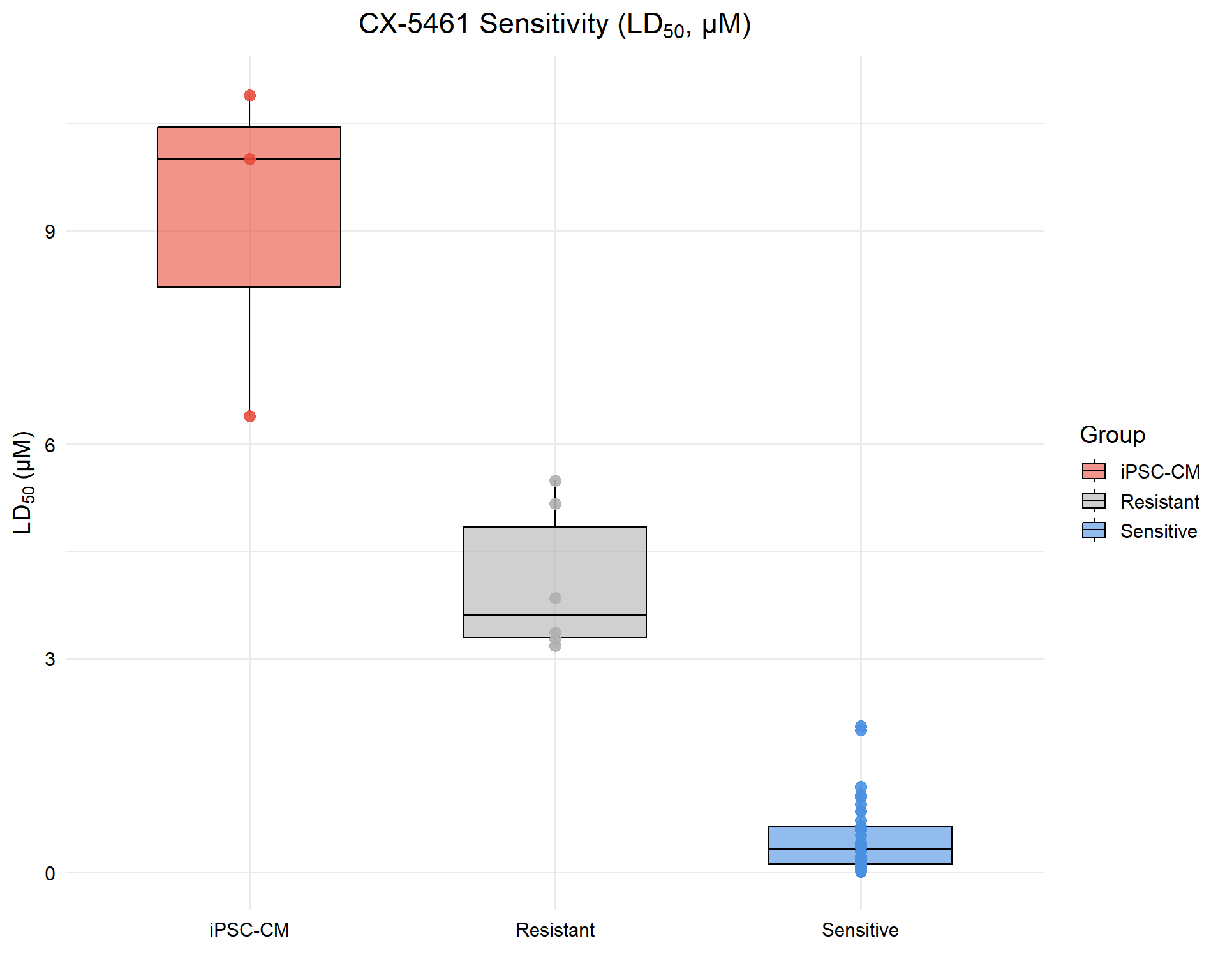
| Version | Author | Date |
|---|---|---|
| 64e2d5a | sayanpaul01 | 2025-10-06 |
📌Elbow plots only — CX-5461 / DOX vs VEH 0.1 & 0.5 µM × 3, 24, 48 h
suppressPackageStartupMessages({
  library(dplyr)
  library(readr)
  library(stringr)
  library(tibble)
  library(tidyr)
})

# ------------------------------------------------------------
# INPUT FILES
# ------------------------------------------------------------
log2cpm_file <- "data/Feature_count_Matrix_Log2CPM_filtered.csv"
meta_file    <- "data/Metadata.csv"

# ------------------------------------------------------------
# LOAD DATA
# ------------------------------------------------------------
log2cpm <- read.csv(log2cpm_file, check.names = FALSE)
colnames(log2cpm) <- gsub("^X", "", trimws(colnames(log2cpm)))

Metadata <- read.csv(meta_file, check.names = FALSE)
Metadata$Sample_name <- gsub("^([0-9]+)\\.([0-9]+)", "\\1-\\2", Metadata$Sample_name)

id_col <- grep("^Entrez|ENTREZ", colnames(log2cpm), value = TRUE)[1]
rownames(log2cpm) <- log2cpm[[id_col]]

# ------------------------------------------------------------
# FUNCTION: plot elbow for one condition
# ------------------------------------------------------------
plot_elbow_one <- function(drug_label = "CX-5461", conc = 0.1, time_h = 3) {
  deg_prefix <- ifelse(drug_label == "CX-5461", "CX", "DOX")
  deg_file <- sprintf("data/DEGs/Toptable_%s_%s_%s.csv", deg_prefix, conc, time_h)

  if (!file.exists(deg_file)) {
    message("Missing DEG file: ", deg_file)
    return()
  }

  deg <- read.csv(deg_file)
  sig <- deg %>% filter(adj.P.Val < 0.05) %>% pull(Entrez_ID) %>% unique()
  if (length(sig) == 0) {
    message("No DEGs in ", deg_file)
    return()
  }

  samples <- Metadata %>%
    filter(Drug %in% c(drug_label, "VEH"),
           Conc. == conc,
           Time == time_h) %>%
    pull(Sample_name)

  matched <- intersect(samples, colnames(log2cpm))
  if (length(matched) == 0) {
    message("No matching samples for ", drug_label, " ", conc, "µM ", time_h, "h")
    return()
  }

  M <- log2cpm[rownames(log2cpm) %in% sig, matched, drop = FALSE]
  M <- as.matrix(M)
  if (nrow(M) < 3) {
    message("Too few genes (<3) for elbow plot: ", drug_label, " ", conc, "µM ", time_h, "h")
    return()
  }

  # ---- K-means elbow ----
  set.seed(123)
  max_k <- min(10, nrow(M) - 1)
  wss <- sapply(1:max_k, function(k)
    kmeans(M, centers = k, nstart = 10, iter.max = 50)$tot.withinss)

  plot(1:max_k, wss, type = "b", pch = 19, col = "darkblue",
       xlab = "Number of Clusters (K)",
       ylab = "Total Within-Cluster SS",
       main = sprintf("Elbow — %s (%.1f µM, %dh) vs VEH", drug_label, conc, time_h))
}

# ------------------------------------------------------------
# EXECUTE — Generate all 12 elbow plots sequentially
# ------------------------------------------------------------

# CX-5461
for (cc in c(0.1, 0.5)) {
  for (tt in c(3, 24, 48)) {
    message(">>> CX-5461 ", cc, " µM ", tt, " h")
    plot_elbow_one("CX-5461", cc, tt)
    dev.flush(); Sys.sleep(1)
  }
}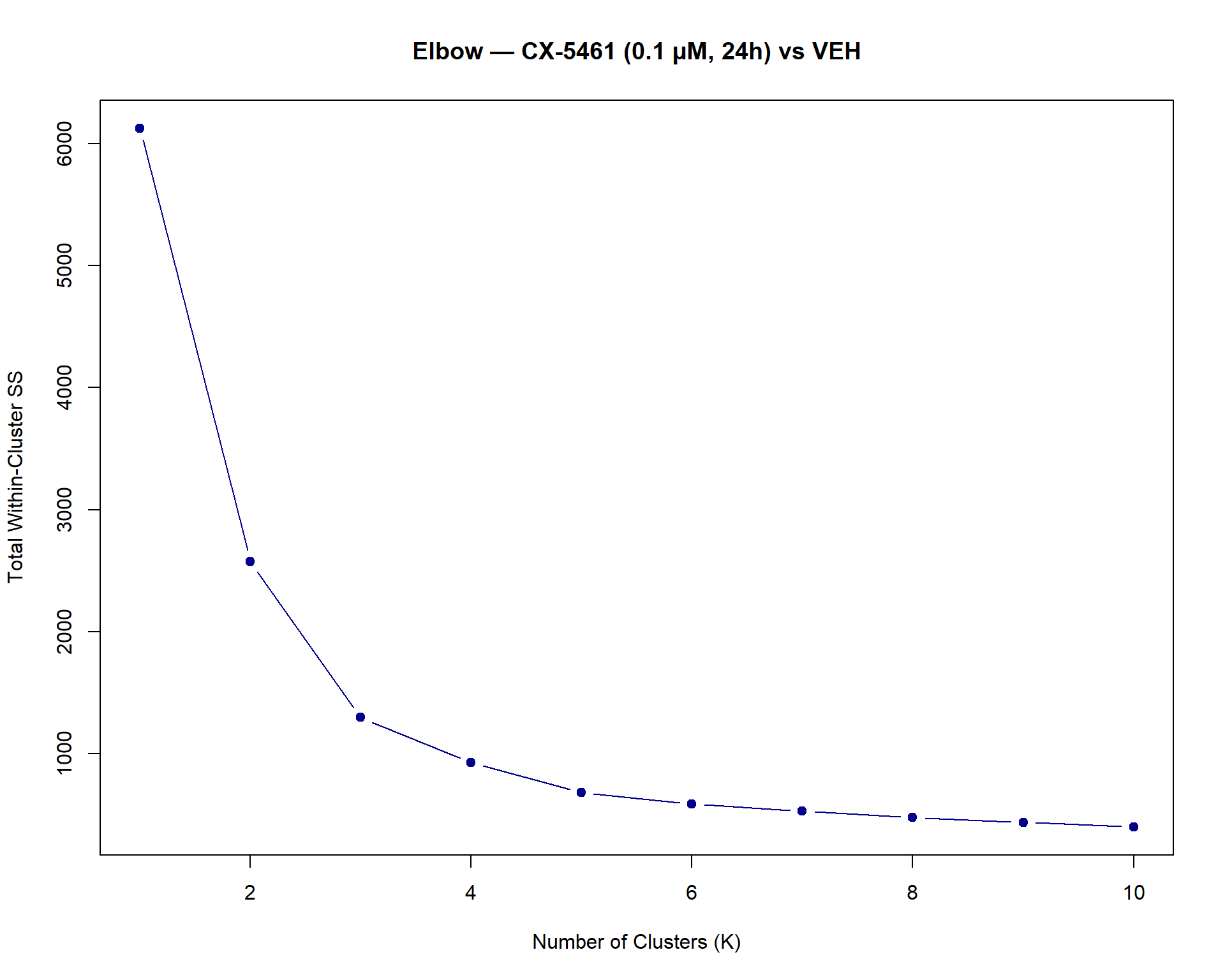
| Version | Author | Date |
|---|---|---|
| 64e2d5a | sayanpaul01 | 2025-10-06 |
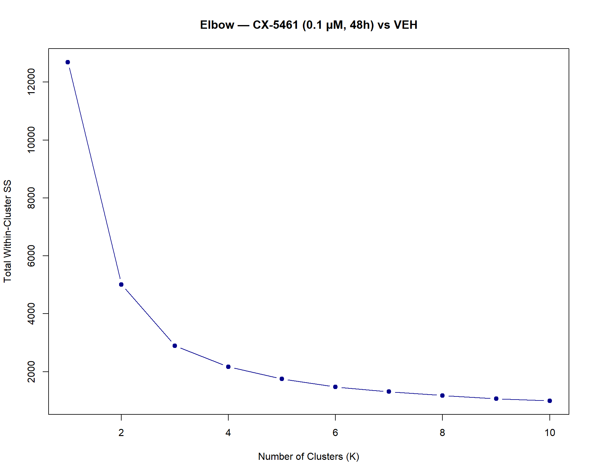
| Version | Author | Date |
|---|---|---|
| 64e2d5a | sayanpaul01 | 2025-10-06 |

| Version | Author | Date |
|---|---|---|
| 64e2d5a | sayanpaul01 | 2025-10-06 |
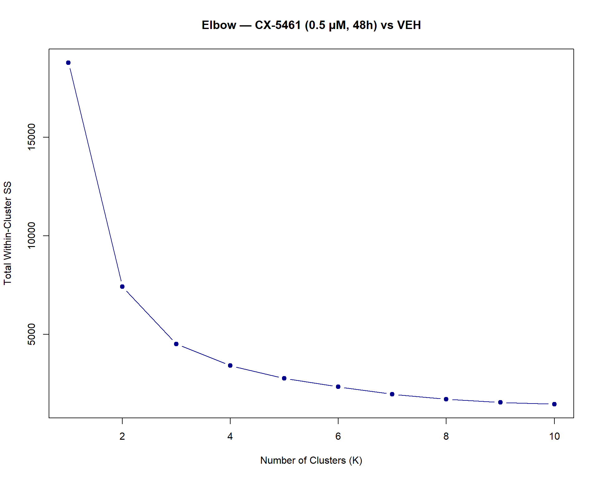
| Version | Author | Date |
|---|---|---|
| 64e2d5a | sayanpaul01 | 2025-10-06 |
# DOX
for (cc in c(0.1, 0.5)) {
  for (tt in c(3, 24, 48)) {
    message(">>> DOX ", cc, " µM ", tt, " h")
    plot_elbow_one("DOX", cc, tt)
    dev.flush(); Sys.sleep(1)
  }
}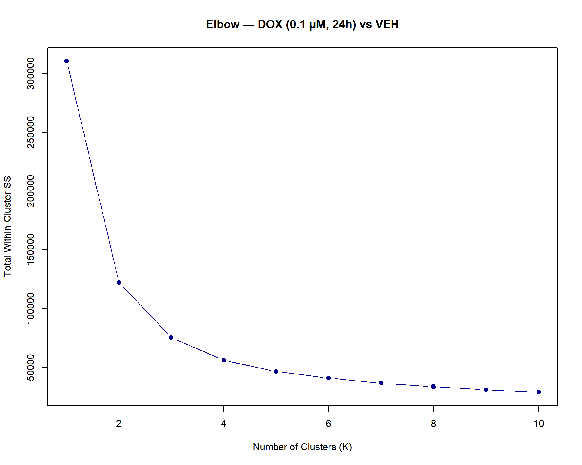
| Version | Author | Date |
|---|---|---|
| 64e2d5a | sayanpaul01 | 2025-10-06 |
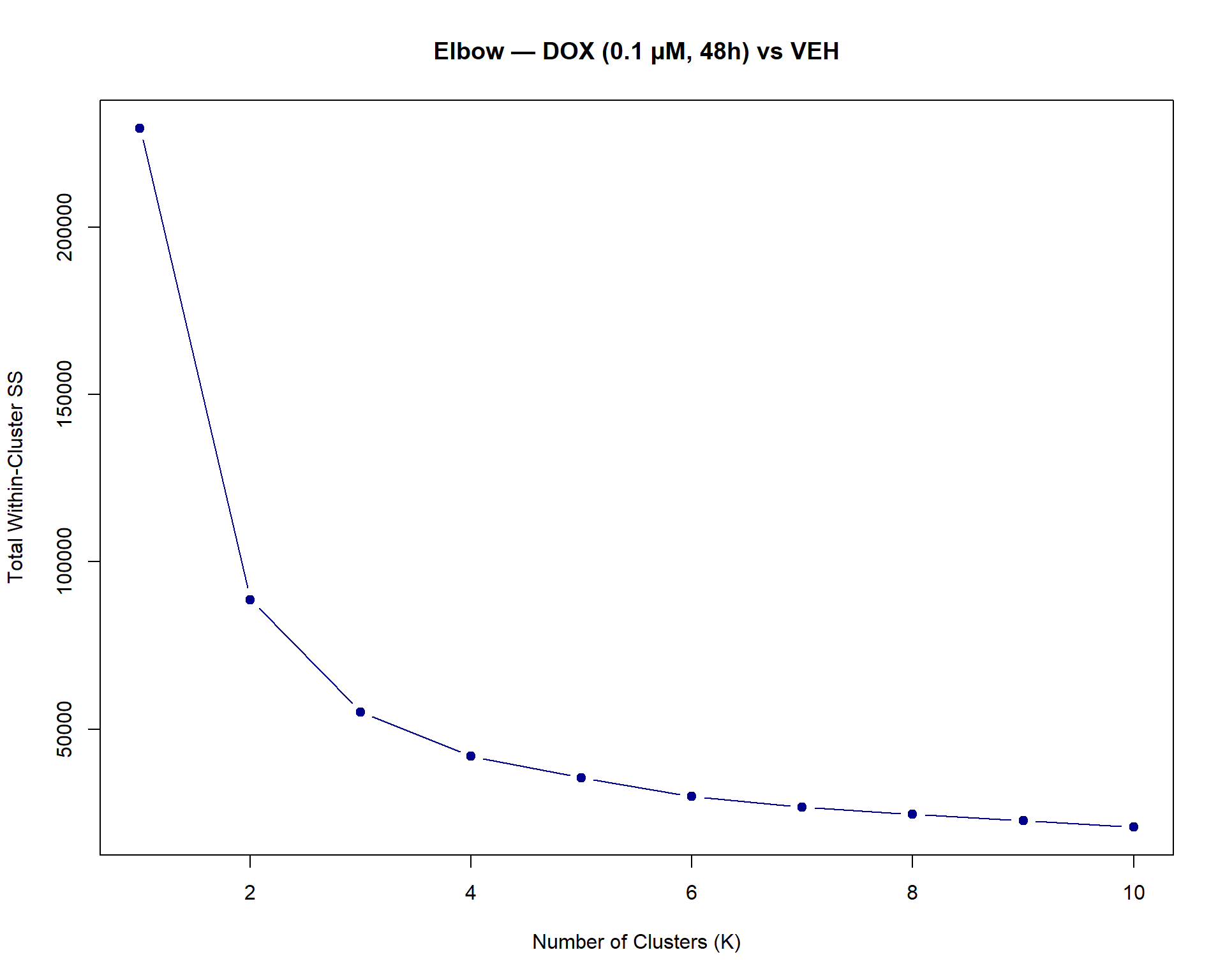
| Version | Author | Date |
|---|---|---|
| 64e2d5a | sayanpaul01 | 2025-10-06 |
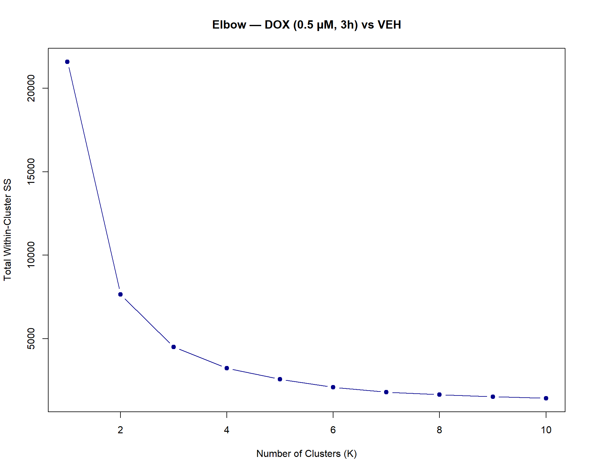
| Version | Author | Date |
|---|---|---|
| 64e2d5a | sayanpaul01 | 2025-10-06 |
Warning: Quick-TRANSfer stage steps exceeded maximum (= 491400)
Warning: Quick-TRANSfer stage steps exceeded maximum (= 491400)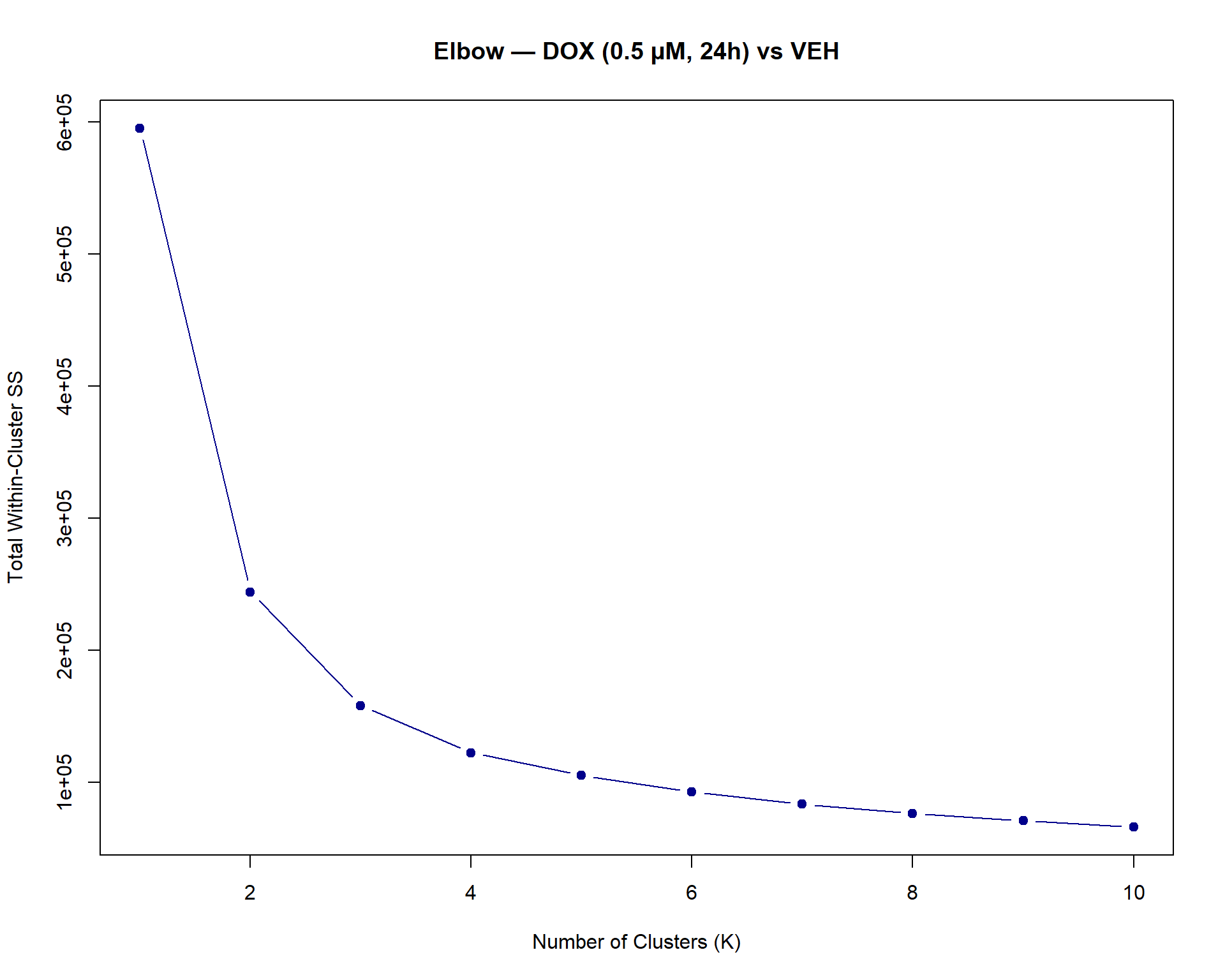
| Version | Author | Date |
|---|---|---|
| 64e2d5a | sayanpaul01 | 2025-10-06 |
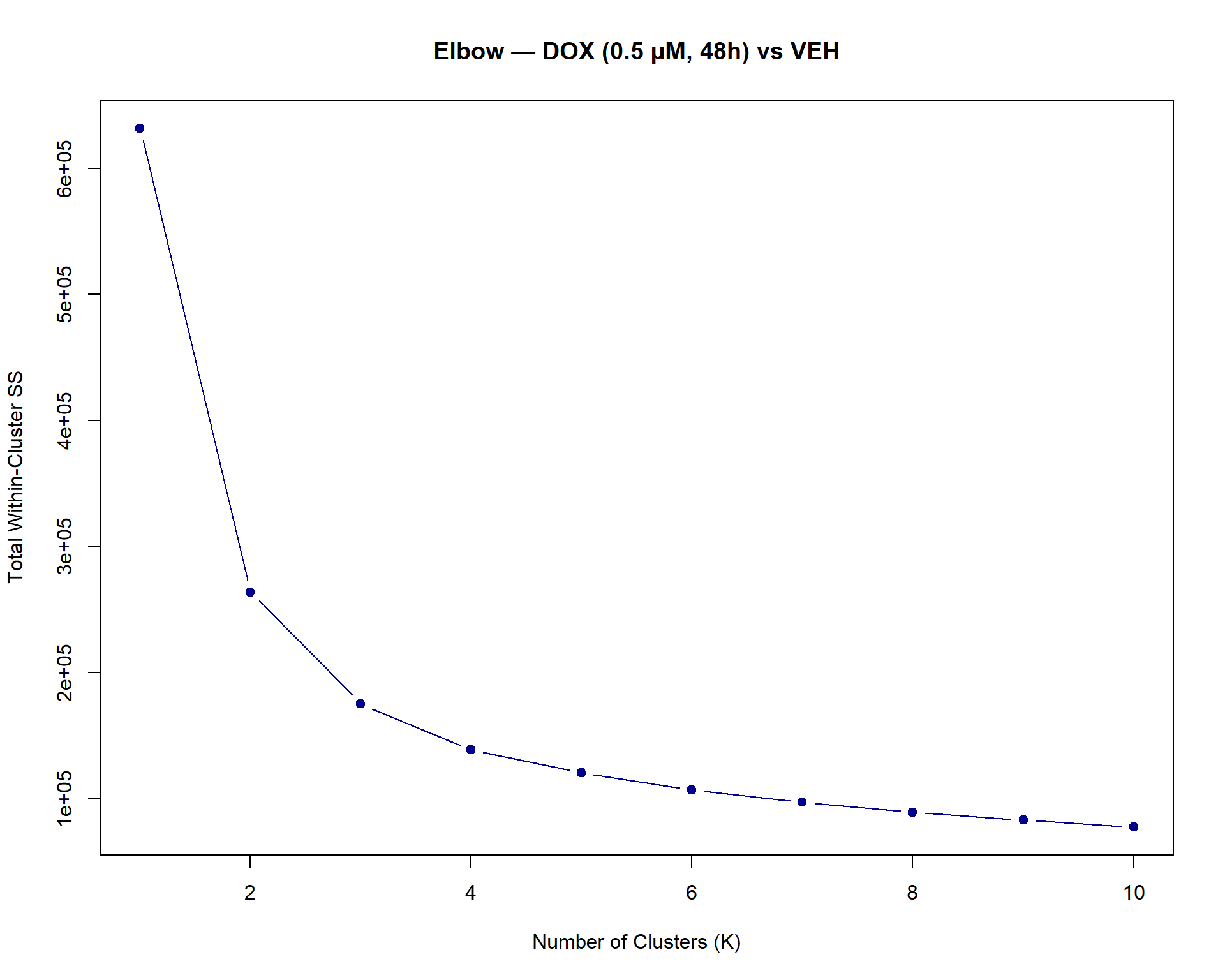
| Version | Author | Date |
|---|---|---|
| 64e2d5a | sayanpaul01 | 2025-10-06 |
📌CX-5461 & DOX vs VEH Heatmaps (0.1 / 0.5 µM ; 3 / 24 / 48 h)
suppressPackageStartupMessages({
  library(ComplexHeatmap)
  library(circlize)
  library(dplyr)
  library(readr)
  library(tibble)
  library(tidyr)
  library(RColorBrewer)
  library(stringr)
})
Warning: package 'ComplexHeatmap' was built under R version 4.3.1Warning: package 'circlize' was built under R version 4.3.3# ------------------------------------------------------------
# INPUT FILES
# ------------------------------------------------------------
log2cpm_file <- "data/Feature_count_Matrix_Log2CPM_filtered.csv"
meta_file <- "data/Metadata.csv"
# ------------------------------------------------------------
# LOAD DATA
# ------------------------------------------------------------
log2cpm <- read.csv(log2cpm_file, check.names = FALSE)
colnames(log2cpm) <- gsub("^X", "", trimws(colnames(log2cpm)))
Metadata <- read.csv(meta_file, check.names = FALSE)
Metadata$Sample_name <- gsub("^([0-9]+)\\.([0-9]+)", "\\1-\\2", Metadata$Sample_name)
id_col <- grep("^Entrez|ENTREZ", colnames(log2cpm), value = TRUE)[1]
rownames(log2cpm) <- log2cpm[[id_col]]
# ------------------------------------------------------------
# COLORS & MAPS
# ------------------------------------------------------------
rename_map <- c("17-3"="1","75-1"="2","84-1"="3","90-1"="4","87-1"="5","78-1"="6")
indv_colors <- setNames(brewer.pal(6, "Dark2"), as.character(1:6))
trt_colors <- c("CX-5461"="#8B006D", "DOX"="#DF707E", "VEH"="#41B333")
conc_colors <- c("0.1"="lightblue", "0.5"="lightcoral")
time_colors <- c("3"="purple", "24"="pink", "48"="tomato3")
cluster_map <- list(
"CX_0.1_3"=NA, "CX_0.1_24"=3, "CX_0.1_48"=3,
"CX_0.5_3"=NA, "CX_0.5_24"=3, "CX_0.5_48"=3,
"DOX_0.1_3"=NA, "DOX_0.1_24"=3, "DOX_0.1_48"=3,
"DOX_0.5_3"=3, "DOX_0.5_24"=3, "DOX_0.5_48"=3
)
# ------------------------------------------------------------
# FUNCTION — DRAW AND SHOW HEATMAP
# ------------------------------------------------------------
plot_heatmap_show <- function(drug_label="CX-5461", conc=0.1, time_h=3) {
deg_prefix <- ifelse(drug_label == "CX-5461", "CX", "DOX")
deg_file <- sprintf("data/DEGs/Toptable_%s_%s_%s.csv", deg_prefix, conc, time_h)
key <- sprintf("%s_%s_%s", deg_prefix, conc, time_h)
row_k <- cluster_map[[key]]
if (!file.exists(deg_file)) {
message("❌ Missing DEG file: ", deg_file)
return()
}
deg <- read.csv(deg_file)
sig <- deg %>% filter(adj.P.Val < 0.05) %>% pull(Entrez_ID) %>% unique()
if (length(sig) == 0) {
message("⚠️ No DEGs for ", key)
return()
}
samples <- Metadata %>%
filter(Drug %in% c(drug_label,"VEH"),
Conc. == conc,
Time == time_h) %>%
pull(Sample_name)
matched <- intersect(samples, colnames(log2cpm))
if (length(matched) == 0) {
message("⚠️ No matching samples for ", key)
return()
}
M <- log2cpm[rownames(log2cpm) %in% sig, matched, drop=FALSE]
if (nrow(M) == 0) {
message("⚠️ Empty matrix for ", key)
return()
}
M <- as.matrix(M)
colnames(M) <- str_replace_all(colnames(M), rename_map)
# --- Annotation
annot_df <- tibble(timeset = colnames(M)) %>%
mutate(sample = timeset) %>%
separate(timeset, into=c("indv","trt","conc","time"), sep="_", remove=FALSE) %>%
mutate(trt=factor(trt,levels=c(drug_label,"VEH")),
indv=factor(indv,levels=as.character(1:6)),
conc=factor(conc,levels=c("0.1","0.5")),
time=factor(time,levels=c("3","24","48"))) %>%
column_to_rownames("sample")
top_ha <- HeatmapAnnotation(
df=annot_df[,c("trt","indv","time")],
col=list(trt=trt_colors, indv=indv_colors, time=time_colors)
)
# --- Color scale
q <- quantile(as.numeric(M), c(0.01, 0.5, 0.99), na.rm=TRUE)
col_fun <- colorRamp2(c(q[1], q[2], q[3]), c("blue","white","red"))
# --- Plotting
message("✅ Displaying: ", key,
ifelse(is.na(row_k), " (no clusters)", paste0(" (k=", row_k, ")")))
if (is.na(row_k)) {
ht <- Heatmap(
M,
top_annotation=top_ha,
show_column_names=TRUE,
show_row_names=FALSE,
cluster_columns=TRUE,
cluster_rows=FALSE,
col=col_fun,
use_raster=TRUE,
raster_device="png",
raster_quality=2,
column_title=sprintf("%s (%.1f µM ; %dh) vs VEH — log2CPM",
drug_label, conc, time_h),
row_title=NULL
)
} else {
ht <- Heatmap(
M,
top_annotation=top_ha,
show_column_names=TRUE,
show_row_names=FALSE,
cluster_columns=TRUE,
cluster_rows=FALSE,
row_km=row_k,
col=col_fun,
use_raster=TRUE,
raster_device="png",
raster_quality=2,
column_title=sprintf("%s (%.1f µM ; %dh) vs VEH — log2CPM",
drug_label, conc, time_h),
row_title="Cluster"
)
}
draw(ht)
}
# ------------------------------------------------------------
# RUN ALL COMBOS
# ------------------------------------------------------------
for (drug in c("CX-5461","DOX")) {
for (cc in c(0.1,0.5)) {
for (tt in c(3,24,48)) {
message("\n>>> ", drug, " ", cc, " µM ", tt, " h")
plot_heatmap_show(drug, cc, tt)
}
}
}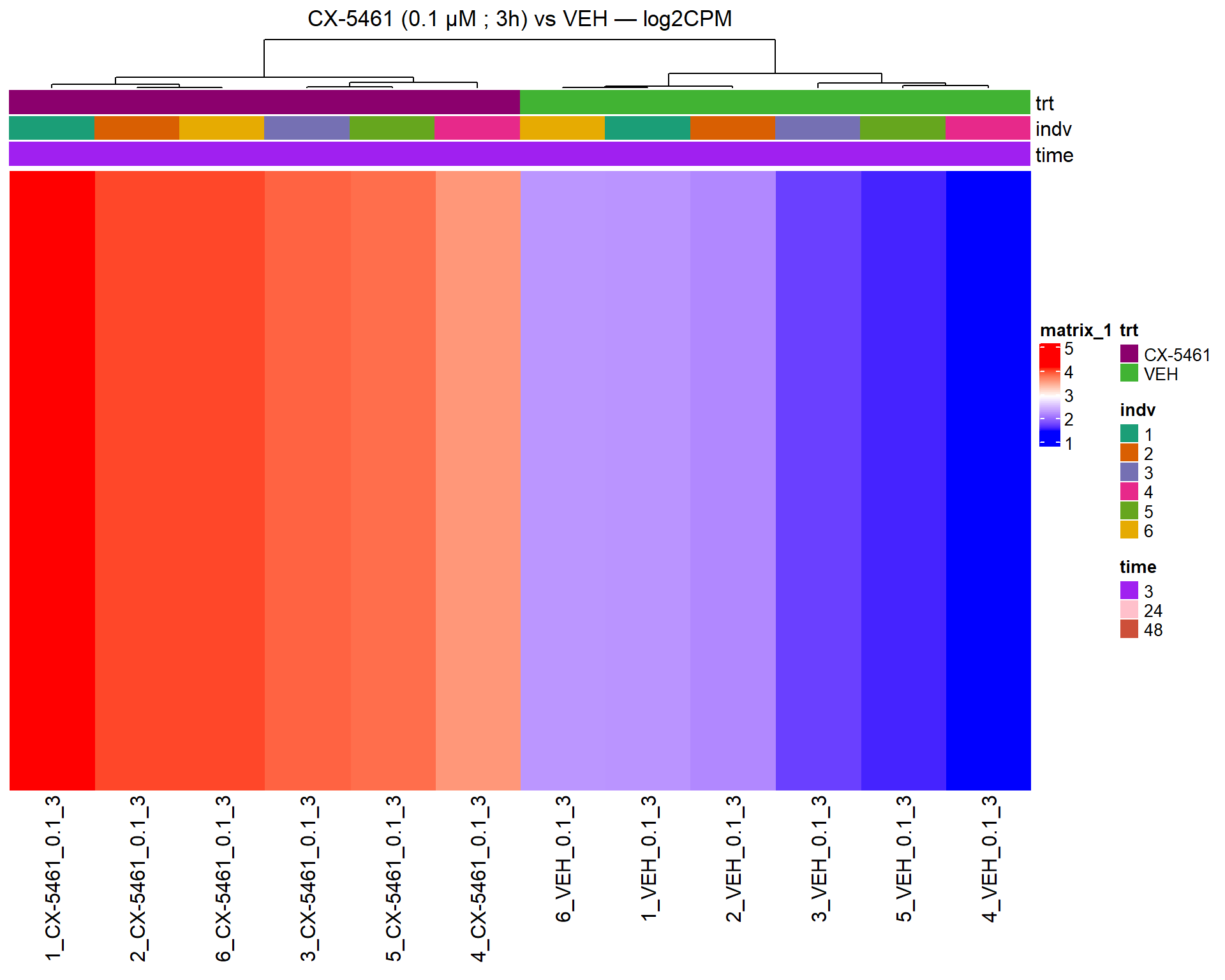
| Version | Author | Date |
|---|---|---|
| 64e2d5a | sayanpaul01 | 2025-10-06 |
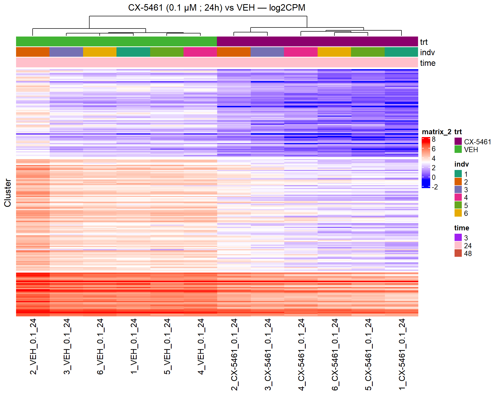
| Version | Author | Date |
|---|---|---|
| 64e2d5a | sayanpaul01 | 2025-10-06 |
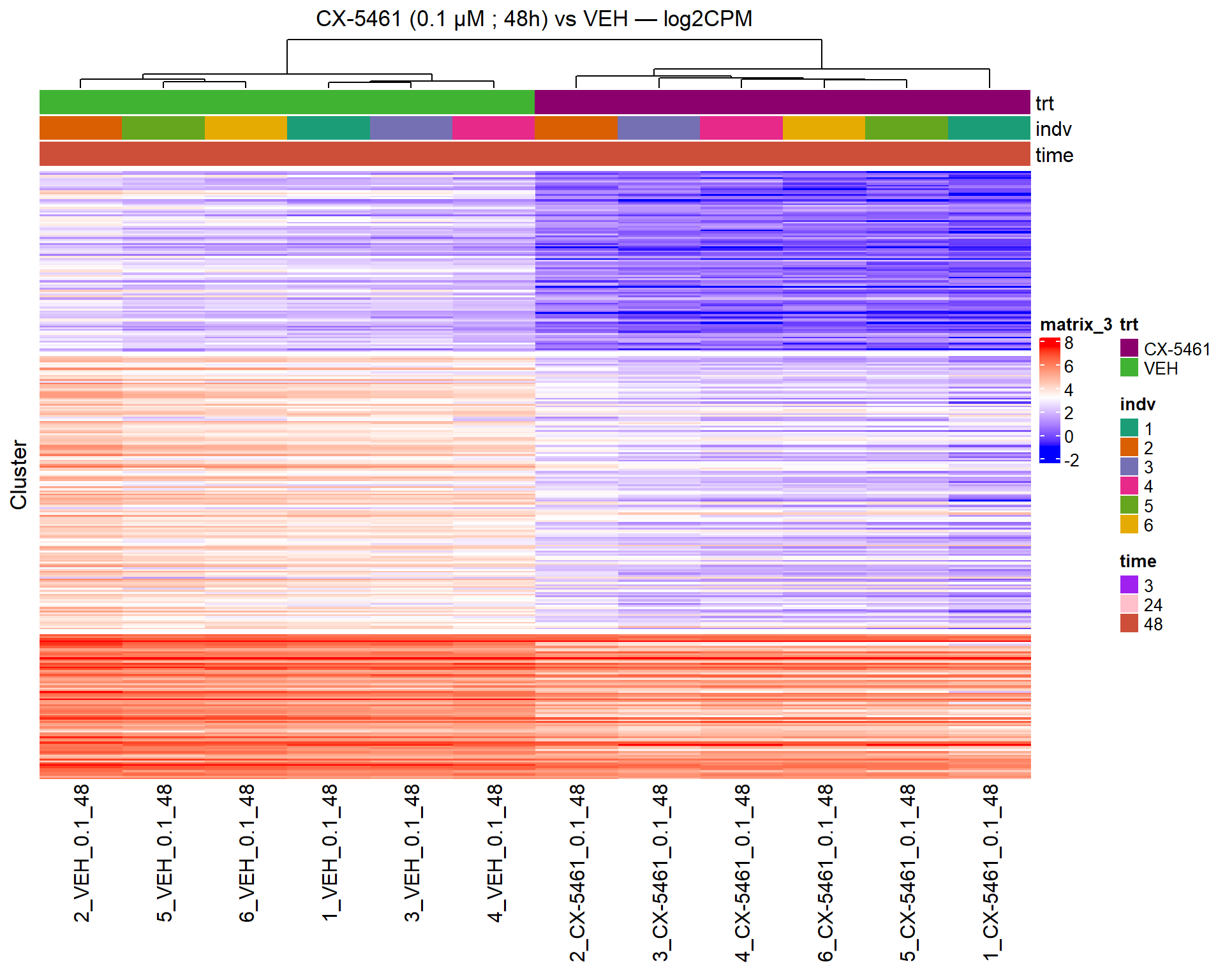
| Version | Author | Date |
|---|---|---|
| 64e2d5a | sayanpaul01 | 2025-10-06 |
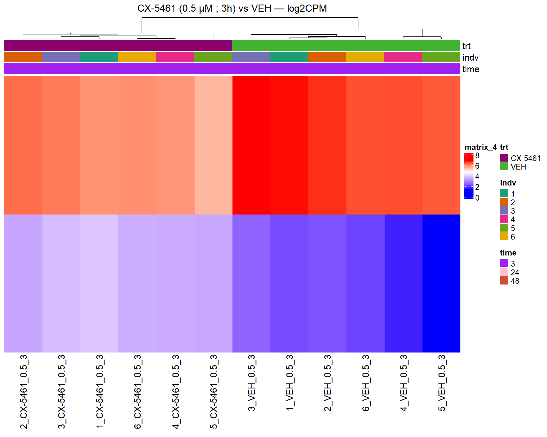
| Version | Author | Date |
|---|---|---|
| 64e2d5a | sayanpaul01 | 2025-10-06 |
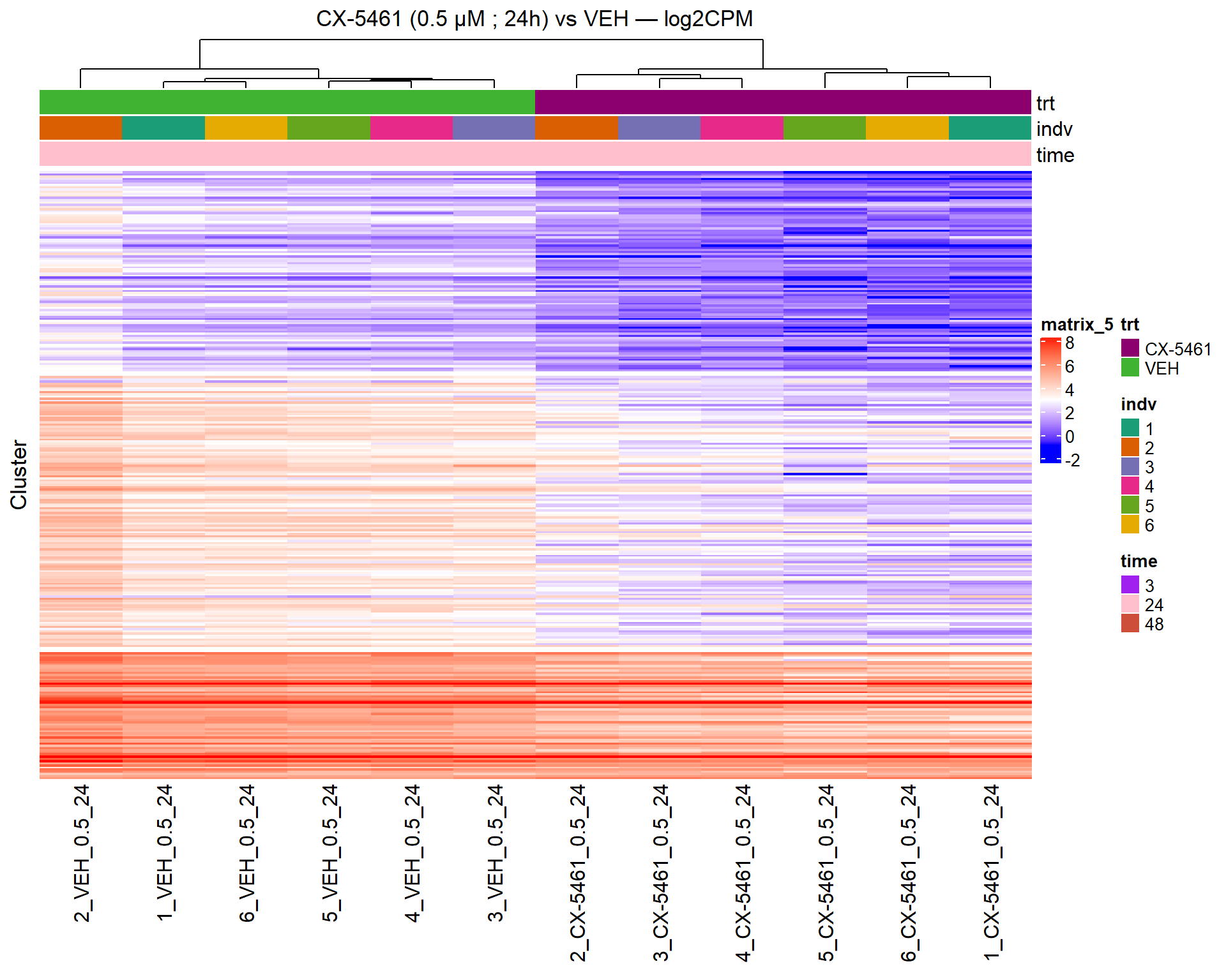
| Version | Author | Date |
|---|---|---|
| 64e2d5a | sayanpaul01 | 2025-10-06 |
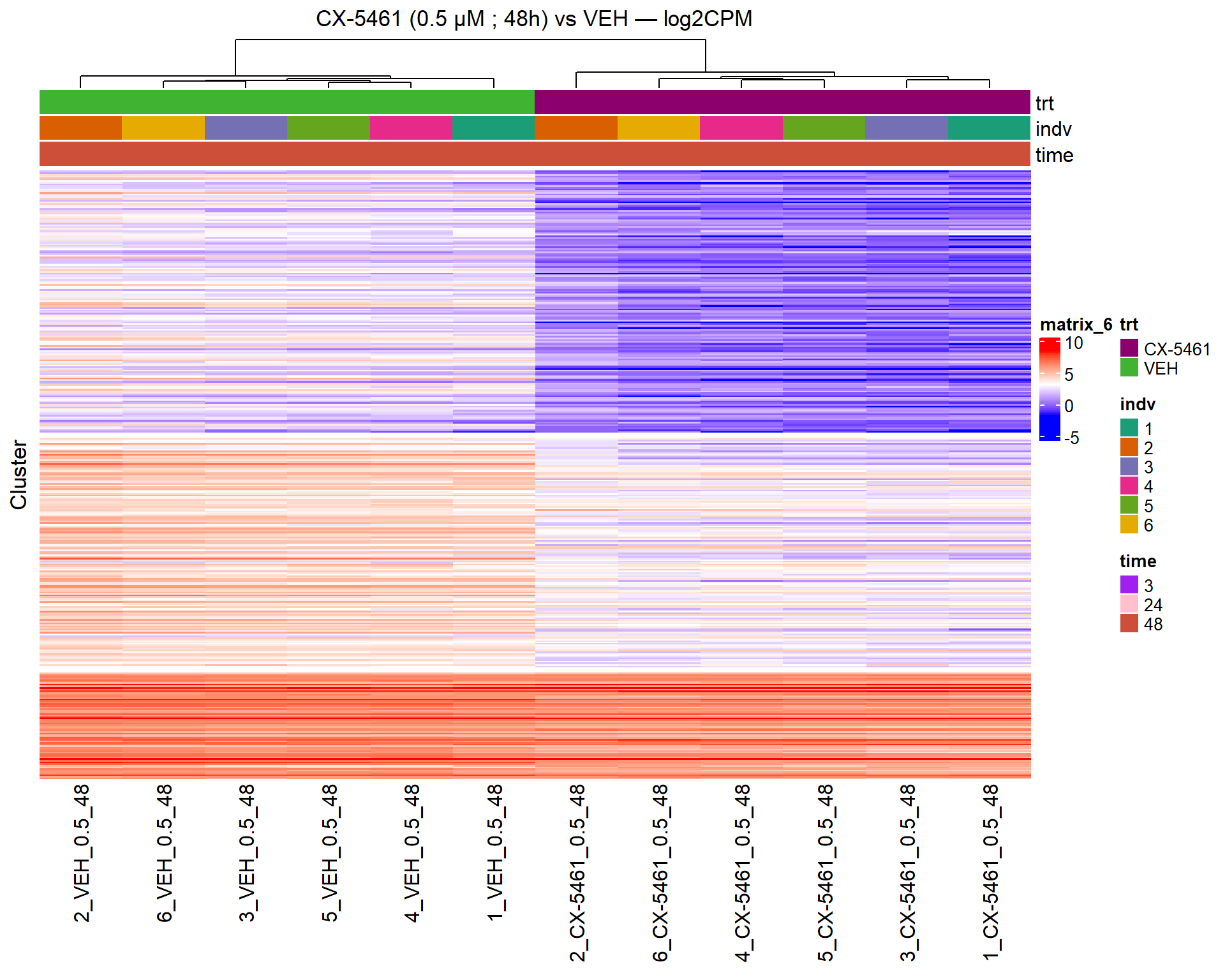
| Version | Author | Date |
|---|---|---|
| 64e2d5a | sayanpaul01 | 2025-10-06 |
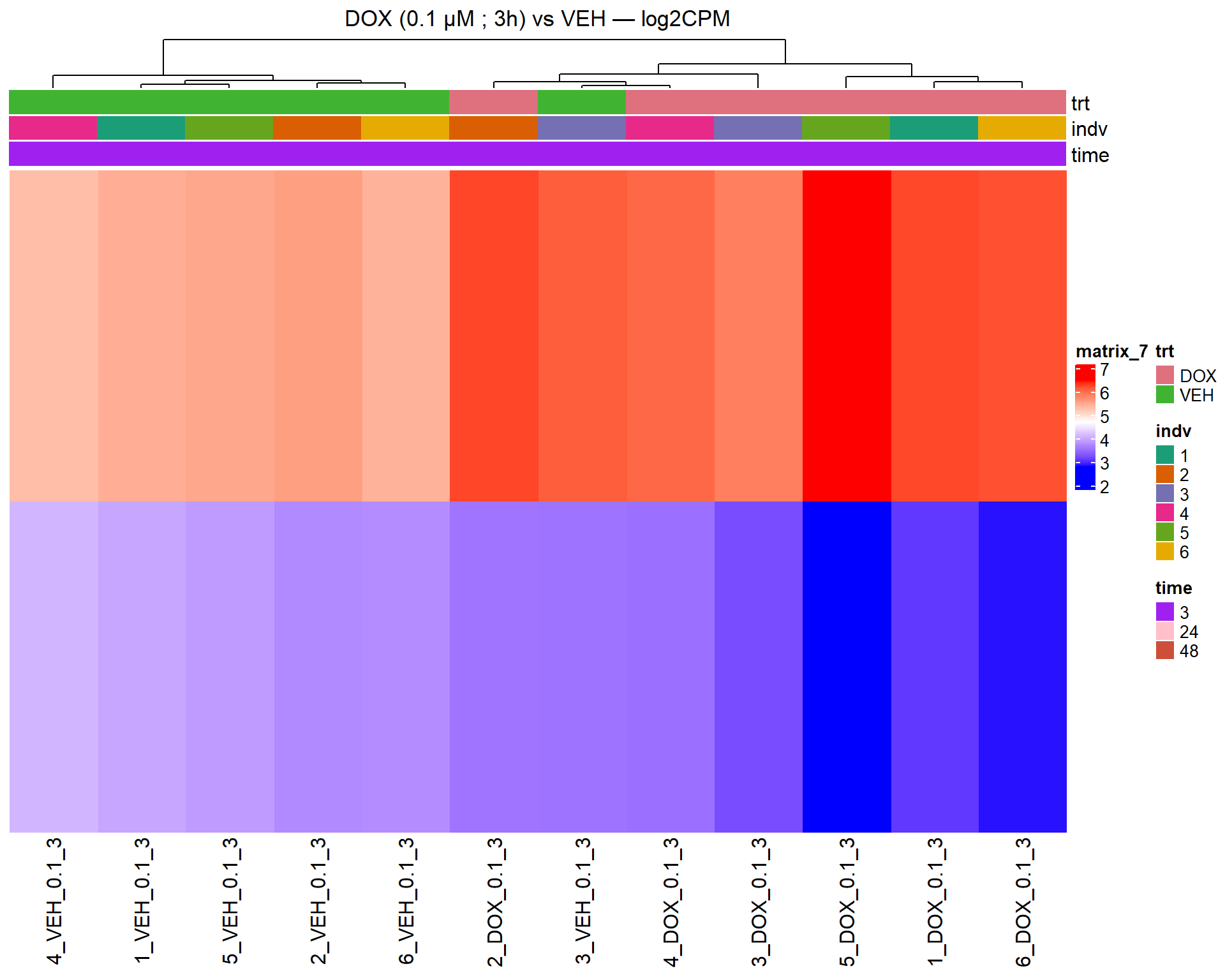
| Version | Author | Date |
|---|---|---|
| 64e2d5a | sayanpaul01 | 2025-10-06 |
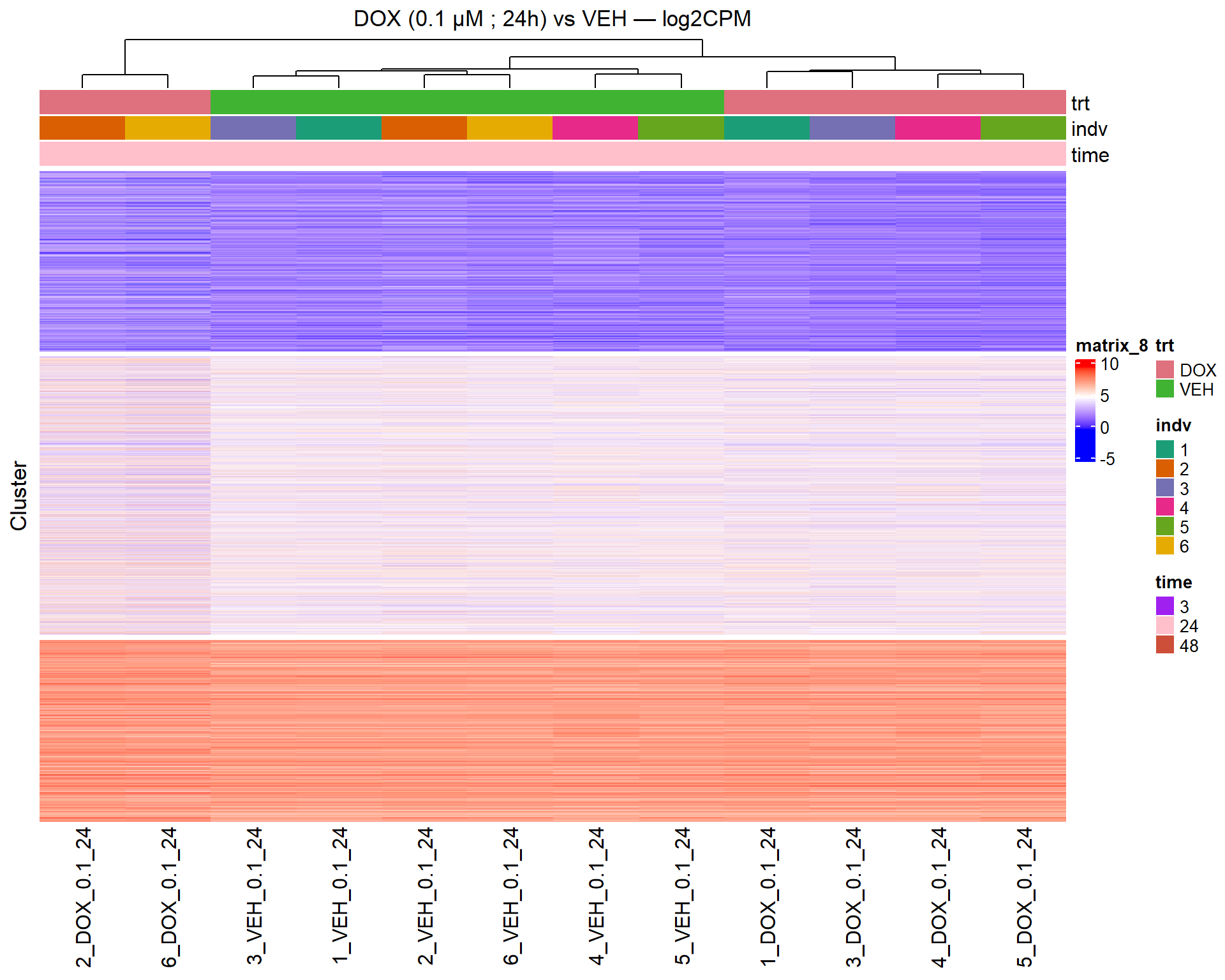
| Version | Author | Date |
|---|---|---|
| 64e2d5a | sayanpaul01 | 2025-10-06 |
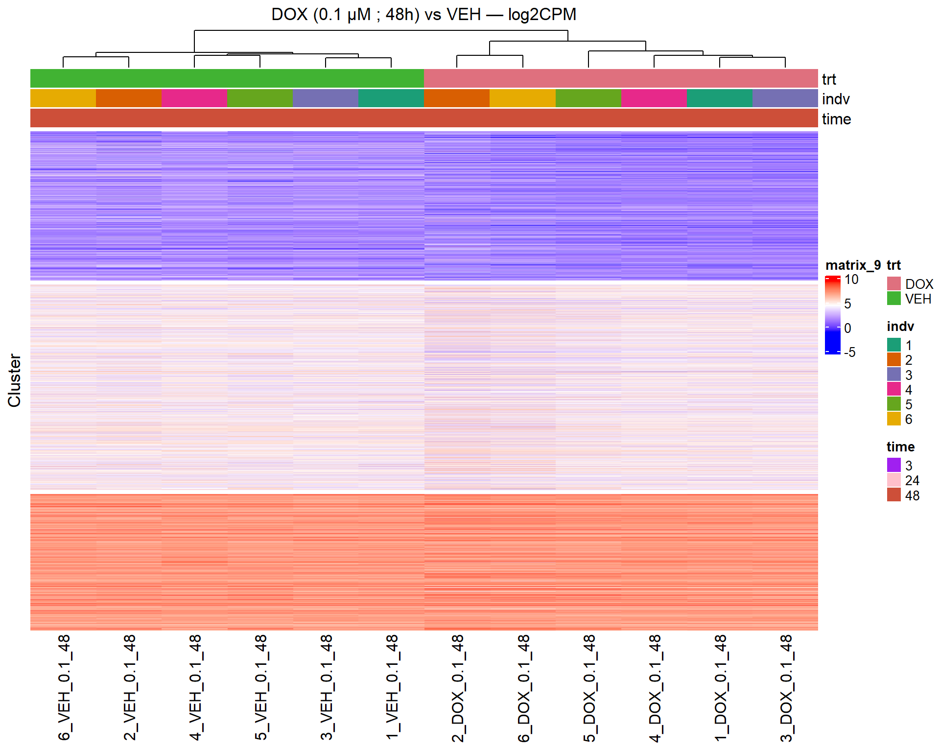
| Version | Author | Date |
|---|---|---|
| 64e2d5a | sayanpaul01 | 2025-10-06 |
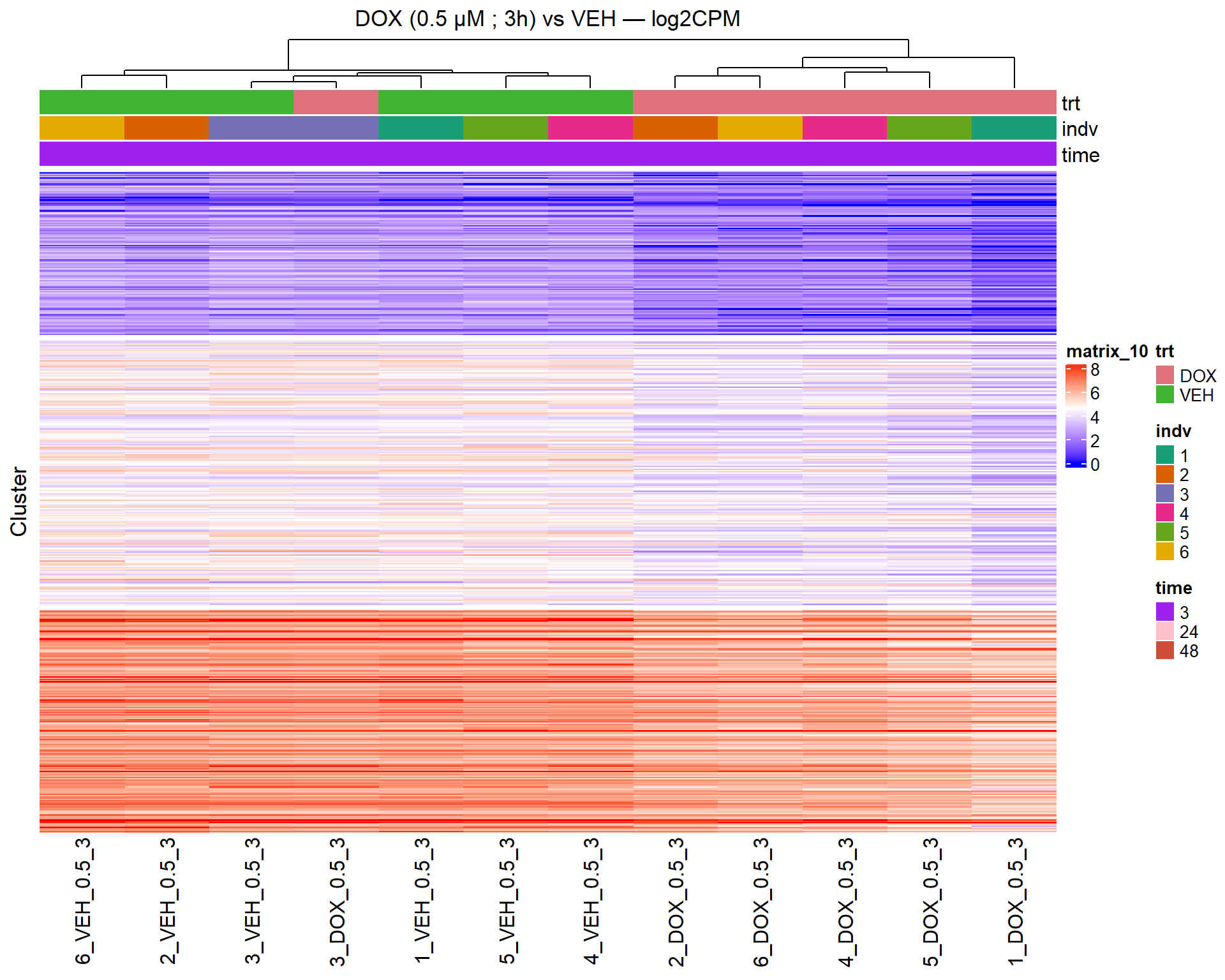
| Version | Author | Date |
|---|---|---|
| 64e2d5a | sayanpaul01 | 2025-10-06 |
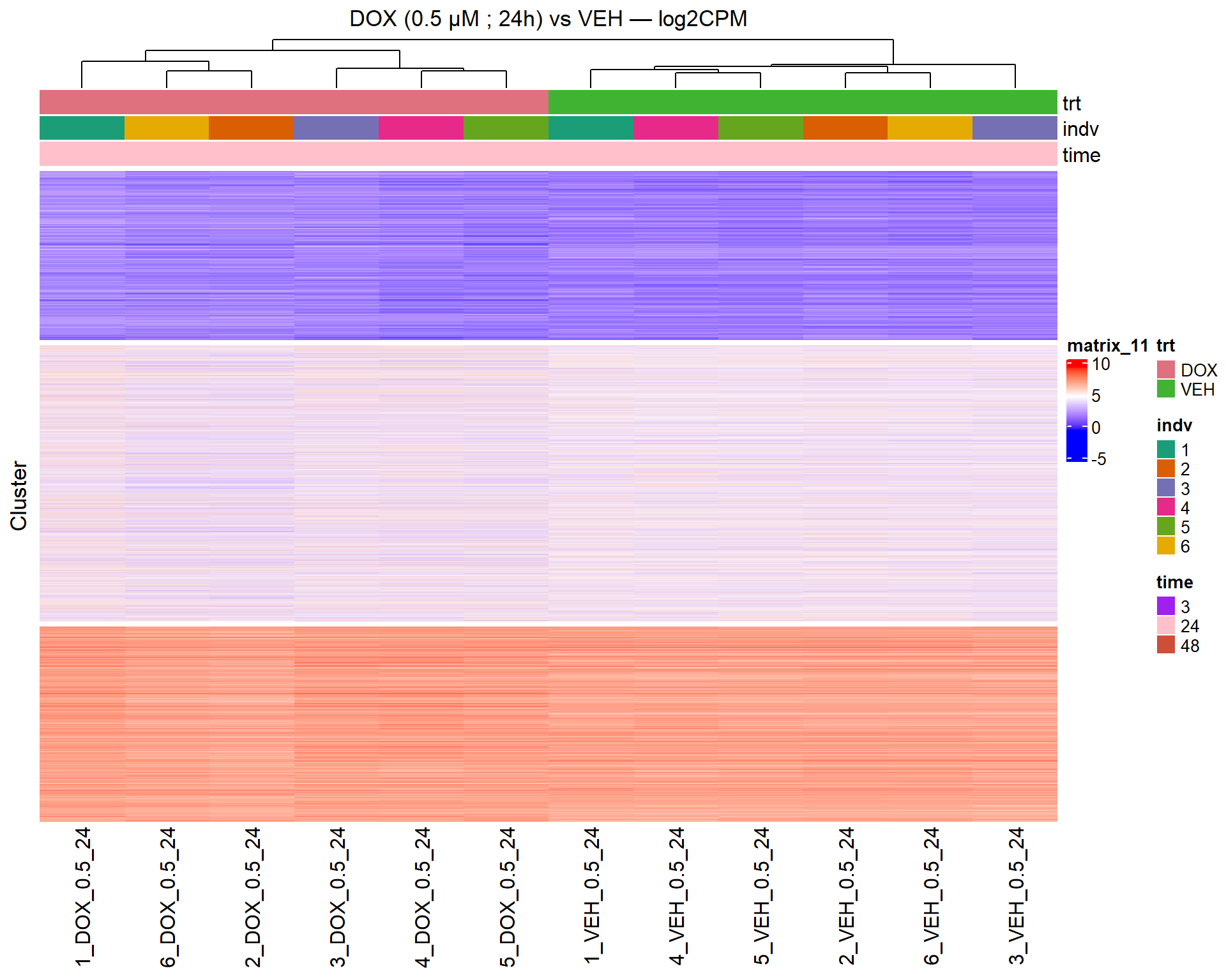
| Version | Author | Date |
|---|---|---|
| 64e2d5a | sayanpaul01 | 2025-10-06 |
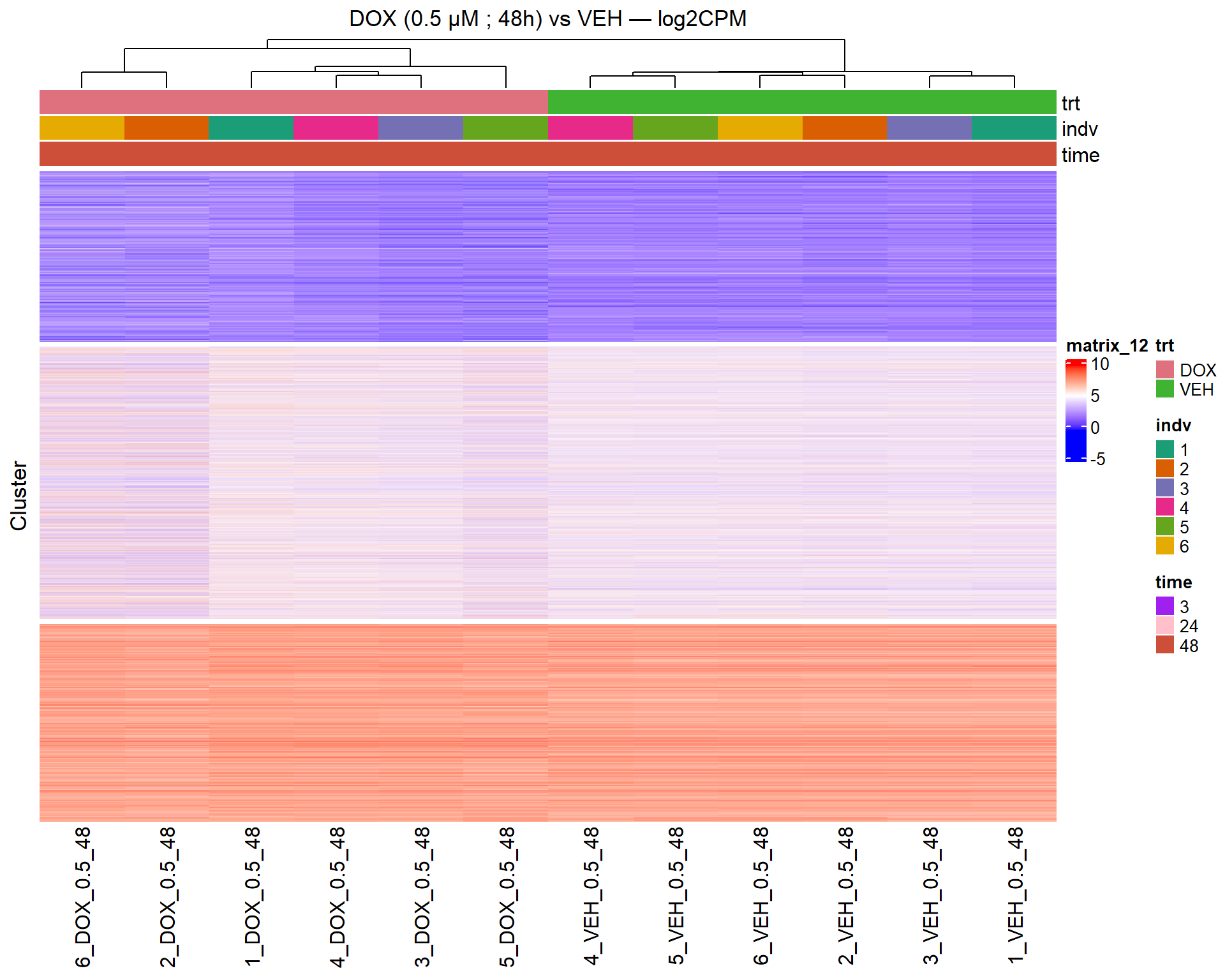
| Version | Author | Date |
|---|---|---|
| 64e2d5a | sayanpaul01 | 2025-10-06 |
message("\n🎨 All heatmaps displayed sequentially.")📌 G-Quadruplex GO Enrichment and Gene Expression
# ======================================================
# 🧬 PART 1: G-QUADRUPLEX GO TERM ENRICHMENT HEATMAP
# ======================================================

library(tidyverse)
library(data.table)
library(ComplexHeatmap)
library(circlize)
library(grid)

# 📁 Define GO enrichment input files
go_files <- list(
  "CX_0.1_3"   = "data/BP/Combined_Terms/GO_All_CX_0.1_3.csv",
  "CX_0.1_24"  = "data/BP/Combined_Terms/GO_All_CX_0.1_24.csv",
  "CX_0.1_48"  = "data/BP/Combined_Terms/GO_All_CX_0.1_48.csv",
  "CX_0.5_3"   = "data/BP/Combined_Terms/GO_All_CX_0.5_3.csv",
  "CX_0.5_24"  = "data/BP/Combined_Terms/GO_All_CX_0.5_24.csv",
  "CX_0.5_48"  = "data/BP/Combined_Terms/GO_All_CX_0.5_48.csv",
  "DOX_0.1_3"  = "data/BP/Combined_Terms/GO_All_DOX_0.1_3.csv",
  "DOX_0.1_24" = "data/BP/Combined_Terms/GO_All_DOX_0.1_24.csv",
  "DOX_0.1_48" = "data/BP/Combined_Terms/GO_All_DOX_0.1_48.csv",
  "DOX_0.5_3"  = "data/BP/Combined_Terms/GO_All_DOX_0.5_3.csv",
  "DOX_0.5_24" = "data/BP/Combined_Terms/GO_All_DOX_0.5_24.csv",
  "DOX_0.5_48" = "data/BP/Combined_Terms/GO_All_DOX_0.5_48.csv"
)

# 🧬 Define G4-related GO terms
g4_terms <- list(
  "GO:0051880" = "G-quadruplex DNA binding",
  "GO:0002151" = "G-quadruplex RNA binding",
  "GO:0071919" = "G-quadruplex DNA formation",
  "GO:1905493" = "Regulation of G-quadruplex DNA binding",
  "GO:0160225" = "G-quadruplex unwinding activity",
  "GO:0061849" = "Telomeric G-quadruplex DNA binding"
)

# 🔍 Function to extract p-values
get_go_values <- function(file_path) {
  df <- fread(file_path)[, .(ID, p.adjust, pvalue)]
  log10pval <- sapply(names(g4_terms), function(go_id) {
    row <- df[ID == go_id]
    if (nrow(row) == 0) return(NA)
    return(-log10(row$pvalue))
  })
  adj_p <- sapply(names(g4_terms), function(go_id) {
    row <- df[ID == go_id]
    if (nrow(row) == 0) return(NA)
    return(row$p.adjust)
  })
  return(list(log10pval = log10pval, adj_p = adj_p))
}

# 🧊 Generate matrices
matrix_list <- map(go_files, get_go_values)
go_matrix <- sapply(matrix_list, function(x) x$log10pval)
padj_matrix <- sapply(matrix_list, function(x) x$adj_p)
rownames(go_matrix) <- unname(unlist(g4_terms))
rownames(padj_matrix) <- rownames(go_matrix)

# 🎨 Define color scale
breaks <- seq(0, 20, by = 2.5)
palette <- colorRampPalette(c("white", "#fde0dd", "#fa9fb5", "#f768a1", "#c51b8a", "#7a0177", "#49006a"))(length(breaks))
col_fun <- colorRamp2(breaks, palette)

# 🔥 Draw heatmap
ht <- Heatmap(
  go_matrix,
  name = "-log10(p value)",
  col = col_fun,
  na_col = "white",
  rect_gp = gpar(col = "black", lwd = 0.5),
  cluster_rows = FALSE,
  cluster_columns = FALSE,
  row_names_gp = gpar(fontsize = 9),
  column_names_gp = gpar(fontsize = 9),
  column_names_rot = 45,
  row_names_max_width = max_text_width(rownames(go_matrix), gp = gpar(fontsize = 9)),
  cell_fun = function(j, i, x, y, width, height, fill) {
    adj_p <- padj_matrix[i, j]
    if (!is.na(adj_p) && adj_p < 0.05) grid.text("*", x, y, gp = gpar(fontsize = 12))
  },
  heatmap_legend_param = list(
    title = "-log10(p value)",
    at = breaks,
    labels = as.character(breaks),
    legend_width = unit(5, "cm"),
    direction = "horizontal",
    title_gp = gpar(fontsize = 10, fontface = "bold"),
    labels_gp = gpar(fontsize = 9)
  )
)

draw(ht, heatmap_legend_side = "top")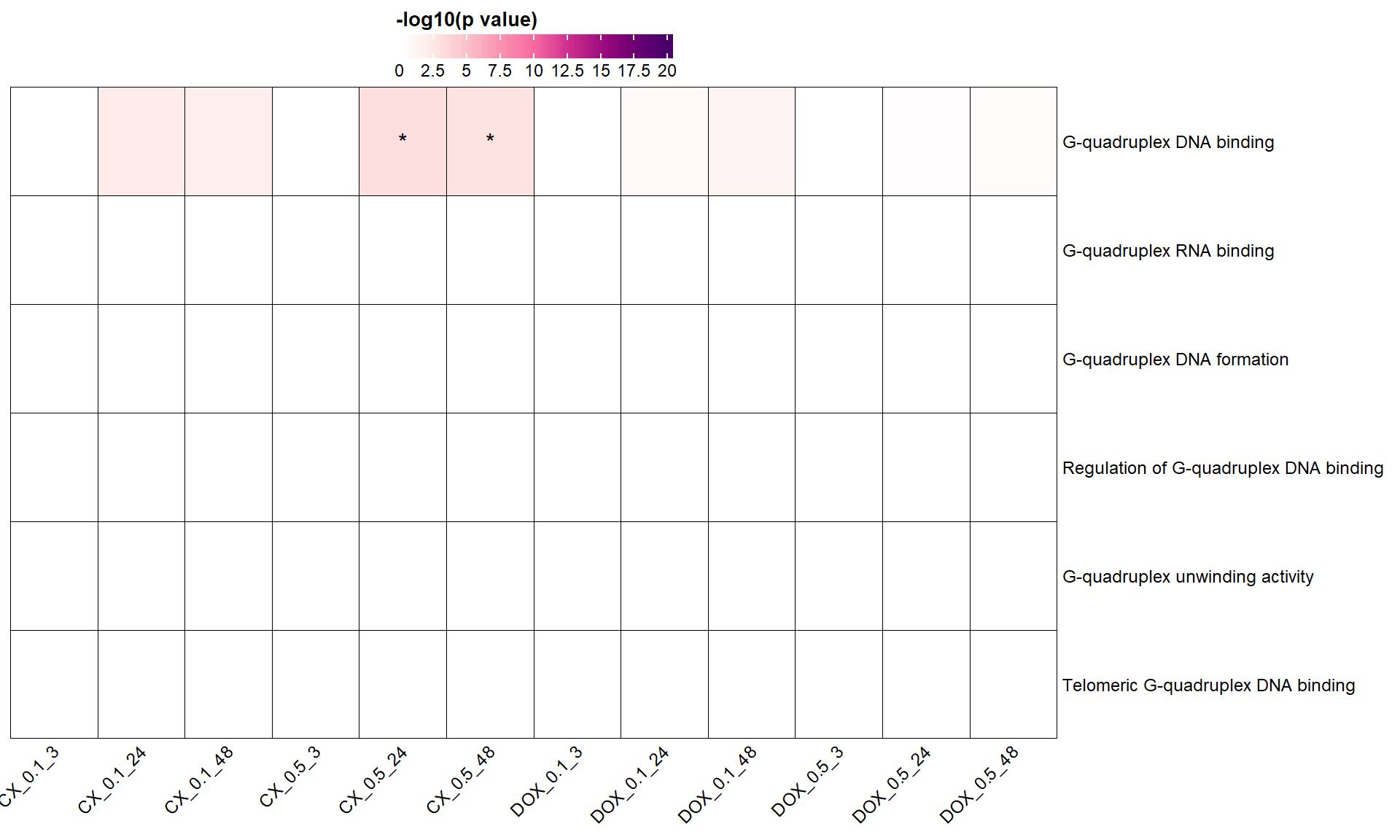
# ======================================================
# 🧬 PART 2: G4-BINDING GENE IDENTIFICATION
# ======================================================

library(org.Hs.eg.db)
library(AnnotationDbi)
library(dplyr)

g4_genes <- AnnotationDbi::select(
  org.Hs.eg.db,
  keys = "GO:0051880",
  columns = c("SYMBOL", "ENTREZID"),
  keytype = "GOALL"
) %>% distinct(SYMBOL, ENTREZID)

g4_genes_vec <- unique(g4_genes$SYMBOL)
g4_genes_vec
[1] "BLM" "DDX11" "NME2" "WRN" "CNBP" "LONP1" "RAD50" "XRN1" "PIF1"
[10] "DHX36"# ======================================================
# 📊 PART 3: LOG2CPM BOXPLOTS FOR G4 GENES
# ======================================================
library(ggplot2)
library(tidyr)
library(clusterProfiler)
library(stringr)
# 📂 Load feature count matrix
boxplot1 <- read.csv("data/Feature_count_Matrix_Log2CPM_filtered.csv") %>% as.data.frame()
colnames(boxplot1) <- trimws(gsub("^X", "", colnames(boxplot1)))
# 🧬 Use G4-binding genes
g4_genes <- g4_genes_vec
# 📄 Load DEG result tables
deg_files <- list.files("data/DEGs", pattern = "Toptable_.*\\.csv", full.names = TRUE)
deg_list <- lapply(deg_files, read.csv)
names(deg_list) <- gsub("data/DEGs/Toptable_|\\.csv", "", deg_files)
# 🧮 Significance checker
is_significant <- function(gene, drug, conc, timepoint) {
condition <- paste(drug, conc, timepoint, sep = "_")
if (!condition %in% names(deg_list)) return(FALSE)
toptable <- deg_list[[condition]]
gene_entrez <- boxplot1$ENTREZID[boxplot1$SYMBOL == gene]
if (length(gene_entrez) == 0) return(FALSE)
any(gene_entrez %in% toptable$Entrez_ID[toptable$adj.P.Val < 0.05])
}
# 🧩 Prepare long-format data per gene
process_gene_data <- function(gene) {
gene_data <- boxplot1 %>% filter(SYMBOL == gene)
long_data <- gene_data %>%
pivot_longer(cols = -c(ENTREZID, SYMBOL, GENENAME), names_to = "Sample", values_to = "log2CPM") %>%
mutate(
Indv = case_when(
grepl("75.1", Sample) ~ "1",
grepl("78.1", Sample) ~ "2",
grepl("87.1", Sample) ~ "3",
grepl("17.3", Sample) ~ "4",
grepl("84.1", Sample) ~ "5",
grepl("90.1", Sample) ~ "6",
TRUE ~ NA_character_
),
Drug = case_when(
grepl("CX.5461", Sample) ~ "CX",
grepl("DOX", Sample) ~ "DOX",
grepl("VEH", Sample) ~ "VEH",
TRUE ~ NA_character_
),
Conc. = case_when(
grepl("_0.1_", Sample) ~ "0.1",
grepl("_0.5_", Sample) ~ "0.5",
TRUE ~ NA_character_
),
Timepoint = case_when(
str_detect(Sample, "_3$") ~ "3",
str_detect(Sample, "_24$") ~ "24",
str_detect(Sample, "_48$") ~ "48",
TRUE ~ NA_character_
),
Condition = paste(Drug, Conc., Timepoint, sep = "_")
)
long_data$Condition <- factor(long_data$Condition, levels = c(
"CX_0.1_3","CX_0.1_24","CX_0.1_48","CX_0.5_3","CX_0.5_24","CX_0.5_48",
"DOX_0.1_3","DOX_0.1_24","DOX_0.1_48","DOX_0.5_3","DOX_0.5_24","DOX_0.5_48",
"VEH_0.1_3","VEH_0.1_24","VEH_0.1_48","VEH_0.5_3","VEH_0.5_24","VEH_0.5_48"
))
significance_labels <- long_data %>%
distinct(Drug, Conc., Timepoint, Condition) %>%
rowwise() %>%
mutate(
max_log2CPM = max(long_data$log2CPM[long_data$Condition == Condition], na.rm = TRUE),
Significance = ifelse(is_significant(gene, Drug, Conc., Timepoint), "*", "")
) %>%
filter(Significance != "") %>% ungroup()
list(long_data = long_data, significance_labels = significance_labels)
}
# 🎨 Plot per gene
for (gene in g4_genes) {
data_info <- process_gene_data(gene)
p <- ggplot(data_info$long_data, aes(x = Condition, y = log2CPM, fill = Drug)) +
geom_boxplot(outlier.shape = NA) +
scale_fill_manual(values = c("CX"="#0000FF","DOX"="#e6d800","VEH"="#FF00FF")) +
geom_point(aes(color = Indv), size = 2, alpha = 0.5, position = position_jitter(width = -1, height = 0)) +
geom_text(data = data_info$significance_labels, aes(x = Condition, y = max_log2CPM + 0.5, label = Significance),
inherit.aes = FALSE, size = 6, color = "black") +
ggtitle(paste("Log2CPM Expression of", gene)) +
labs(x = "Treatment", y = "log2CPM") +
theme_bw() +
theme(plot.title = element_text(size = rel(2), hjust = 0.5),
axis.title = element_text(size = 15, color = "black"),
axis.text.x = element_text(size = 10, color = "black", angle = 90, hjust = 1))
print(p)
}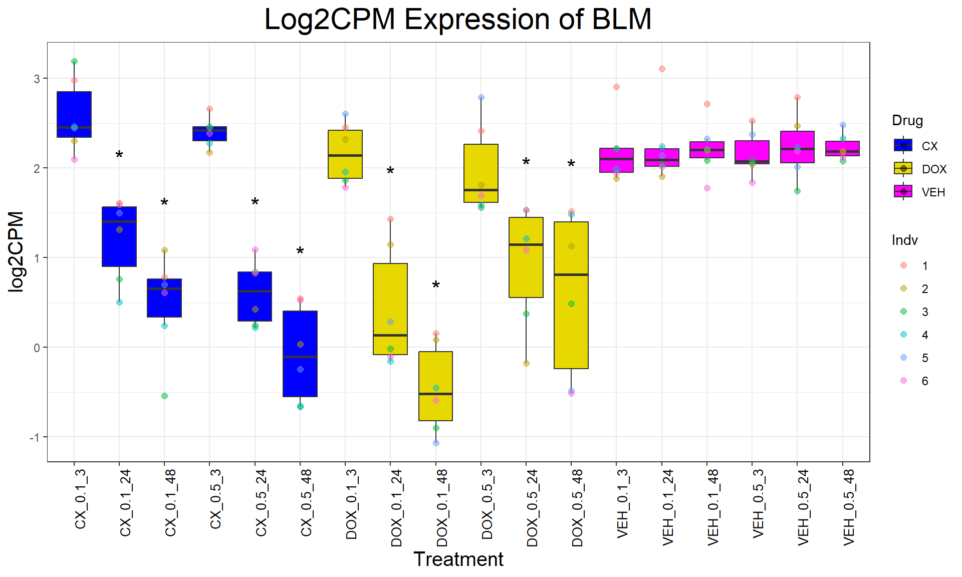
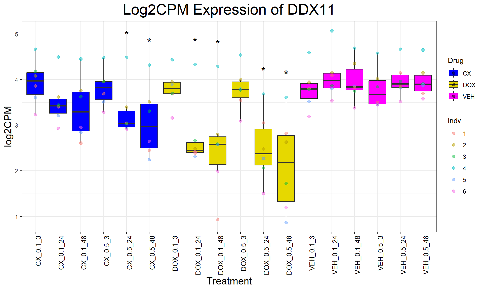
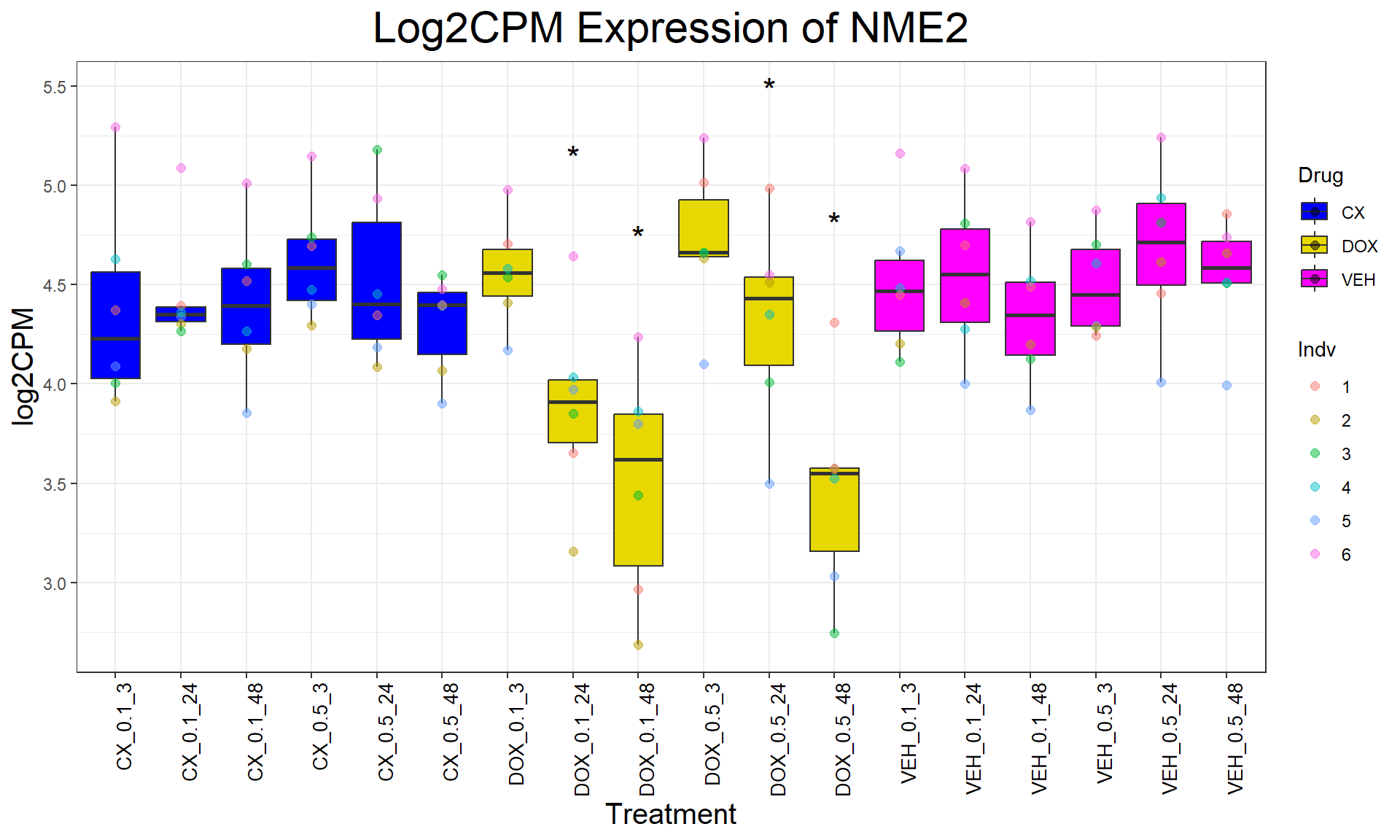
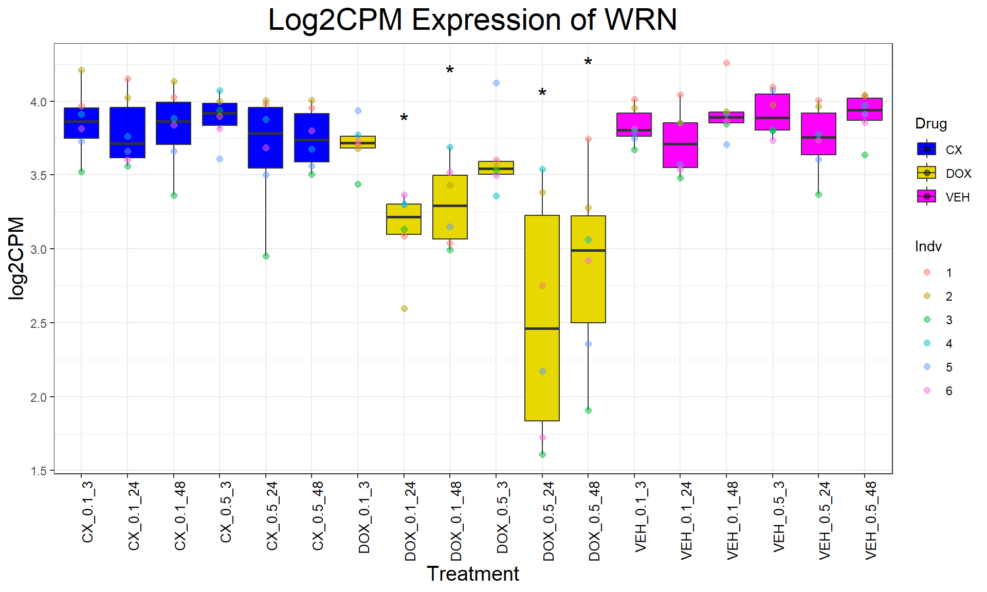
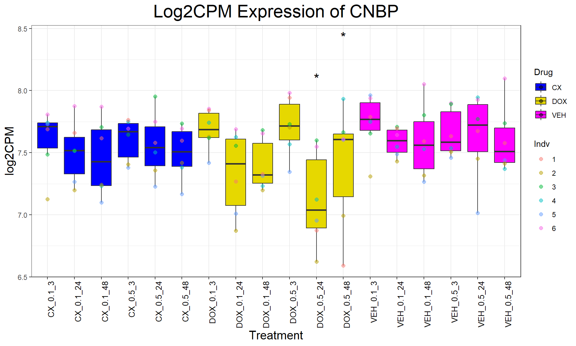
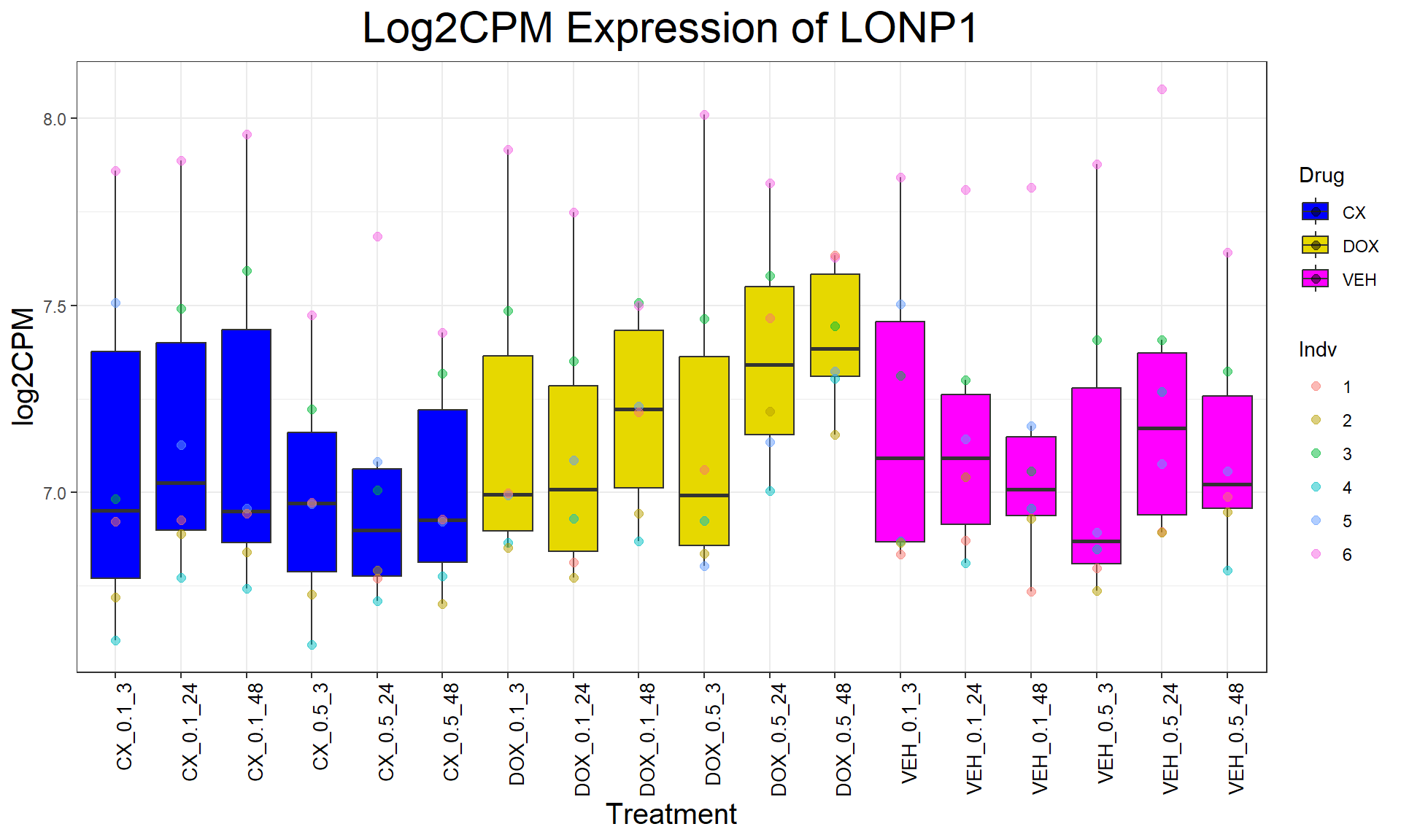
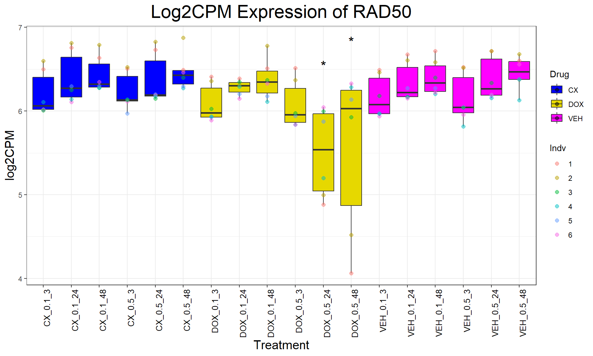
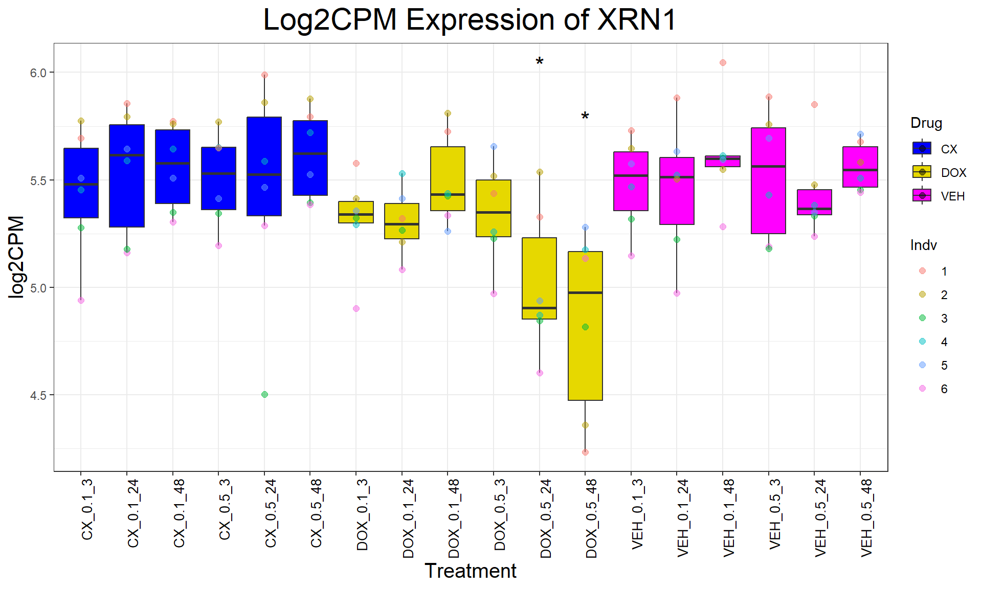
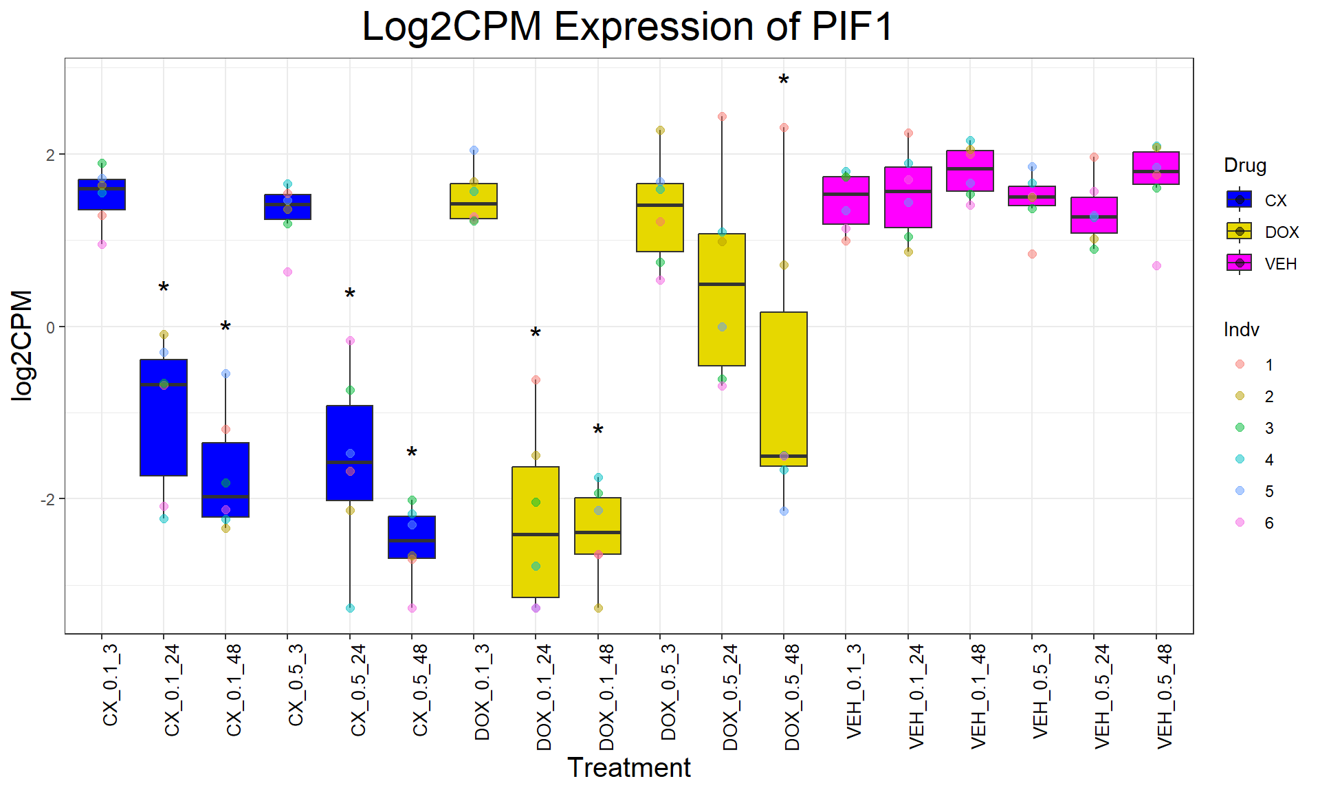
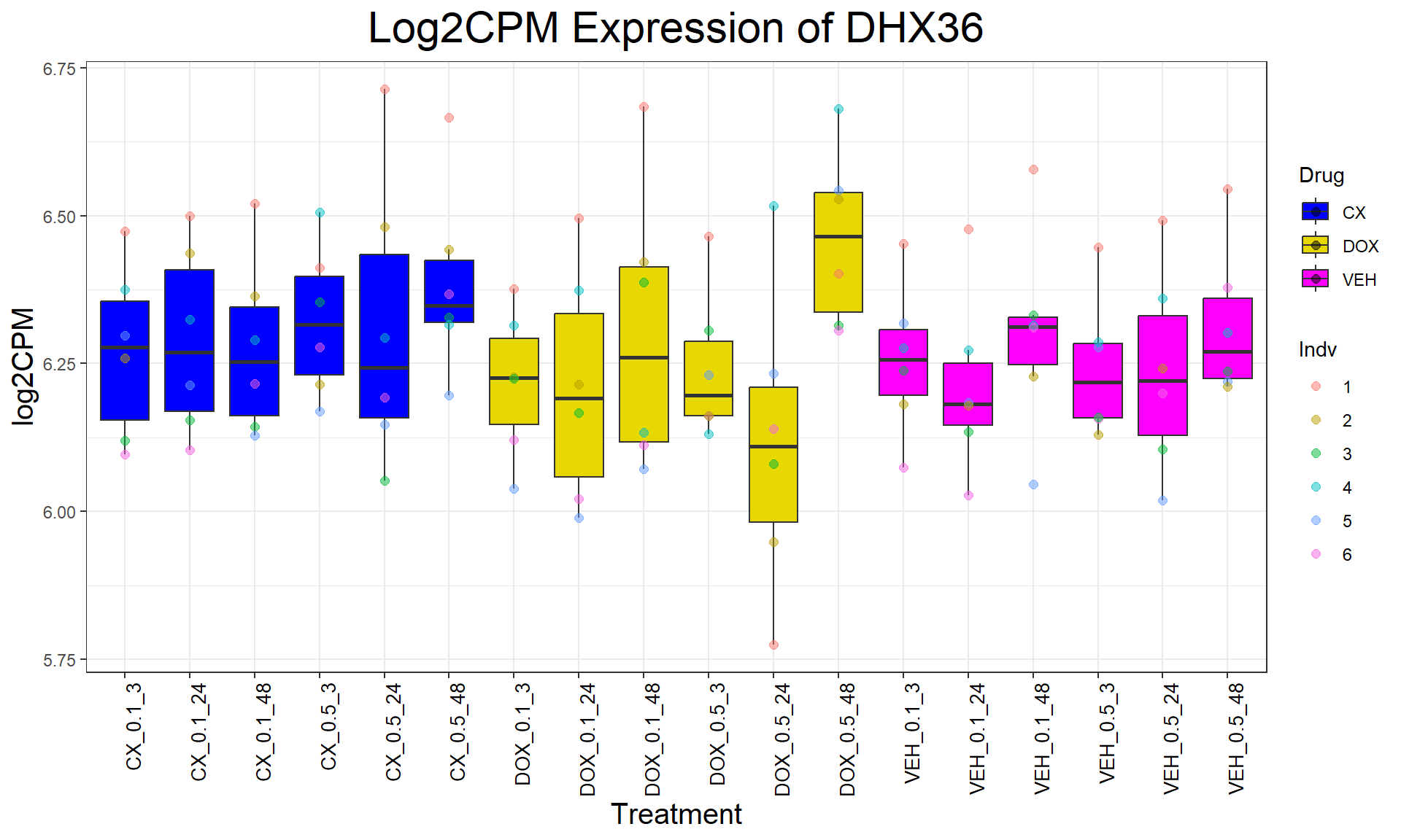
sessionInfo()R version 4.3.0 (2023-04-21 ucrt)
Platform: x86_64-w64-mingw32/x64 (64-bit)
Running under: Windows 11 x64 (build 26100)
Matrix products: default
locale:
[1] LC_COLLATE=English_United States.utf8
[2] LC_CTYPE=English_United States.utf8
[3] LC_MONETARY=English_United States.utf8
[4] LC_NUMERIC=C
[5] LC_TIME=English_United States.utf8
time zone: America/Chicago
tzcode source: internal
attached base packages:
[1] grid stats4 stats graphics grDevices utils datasets
[8] methods base
other attached packages:
[1] clusterProfiler_4.10.1 data.table_1.17.0 RColorBrewer_1.1-3
[4] circlize_0.4.16 ComplexHeatmap_2.18.0 lubridate_1.9.4
[7] forcats_1.0.0 stringr_1.5.1 purrr_1.0.4
[10] readr_2.1.5 tidyverse_2.0.0 org.Hs.eg.db_3.18.0
[13] AnnotationDbi_1.64.1 IRanges_2.36.0 S4Vectors_0.40.2
[16] Biobase_2.62.0 BiocGenerics_0.48.1 ggplot2_3.5.2
[19] tibble_3.2.1 tidyr_1.3.1 dplyr_1.1.4
loaded via a namespace (and not attached):
[1] rstudioapi_0.17.1 jsonlite_2.0.0 shape_1.4.6.1
[4] magrittr_2.0.3 magick_2.8.6 farver_2.1.2
[7] rmarkdown_2.29 GlobalOptions_0.1.2 fs_1.6.3
[10] zlibbioc_1.48.2 vctrs_0.6.5 memoise_2.0.1
[13] Cairo_1.6-2 RCurl_1.98-1.17 ggtree_3.10.1
[16] htmltools_0.5.8.1 gridGraphics_0.5-1 sass_0.4.10
[19] bslib_0.9.0 plyr_1.8.9 cachem_1.1.0
[22] whisker_0.4.1 igraph_2.1.4 lifecycle_1.0.4
[25] iterators_1.0.14 pkgconfig_2.0.3 gson_0.1.0
[28] Matrix_1.6-1.1 R6_2.6.1 fastmap_1.2.0
[31] GenomeInfoDbData_1.2.11 clue_0.3-66 digest_0.6.34
[34] aplot_0.2.5 enrichplot_1.22.0 colorspace_2.1-0
[37] patchwork_1.3.0 rprojroot_2.0.4 RSQLite_2.3.9
[40] labeling_0.4.3 timechange_0.3.0 httr_1.4.7
[43] polyclip_1.10-7 mgcv_1.9-3 compiler_4.3.0
[46] bit64_4.6.0-1 withr_3.0.2 doParallel_1.0.17
[49] BiocParallel_1.36.0 viridis_0.6.5 DBI_1.2.3
[52] ggforce_0.4.2 MASS_7.3-60 rjson_0.2.23
[55] HDO.db_0.99.1 tools_4.3.0 scatterpie_0.2.4
[58] ape_5.8-1 httpuv_1.6.15 glue_1.7.0
[61] nlme_3.1-168 GOSemSim_2.28.1 promises_1.3.2
[64] shadowtext_0.1.4 cluster_2.1.8.1 reshape2_1.4.4
[67] fgsea_1.28.0 generics_0.1.3 gtable_0.3.6
[70] tzdb_0.5.0 hms_1.1.3 tidygraph_1.3.1
[73] XVector_0.42.0 ggrepel_0.9.6 foreach_1.5.2
[76] pillar_1.10.2 yulab.utils_0.2.0 later_1.3.2
[79] splines_4.3.0 tweenr_2.0.3 treeio_1.26.0
[82] lattice_0.22-7 bit_4.6.0 tidyselect_1.2.1
[85] GO.db_3.18.0 Biostrings_2.70.3 knitr_1.50
[88] git2r_0.36.2 gridExtra_2.3 xfun_0.52
[91] graphlayouts_1.2.2 matrixStats_1.5.0 stringi_1.8.3
[94] lazyeval_0.2.2 workflowr_1.7.1 ggfun_0.1.8
[97] yaml_2.3.10 evaluate_1.0.3 codetools_0.2-20
[100] ggraph_2.2.1 qvalue_2.34.0 ggplotify_0.1.2
[103] cli_3.6.1 munsell_0.5.1 jquerylib_0.1.4
[106] Rcpp_1.0.12 GenomeInfoDb_1.38.8 png_0.1-8
[109] parallel_4.3.0 blob_1.2.4 DOSE_3.28.2
[112] bitops_1.0-9 viridisLite_0.4.2 tidytree_0.4.6
[115] scales_1.3.0 crayon_1.5.3 GetoptLong_1.0.5
[118] rlang_1.1.3 cowplot_1.1.3 fastmatch_1.1-6
[121] KEGGREST_1.42.0