Figure 8: DOX response eGenes are enriched amongst TOP2i response genes.
ERM
2023-09-28
Last updated: 2023-09-28
Checks: 7 0
Knit directory: Cardiotoxicity/
This reproducible R Markdown analysis was created with workflowr (version 1.7.1). The Checks tab describes the reproducibility checks that were applied when the results were created. The Past versions tab lists the development history.
Great! Since the R Markdown file has been committed to the Git repository, you know the exact version of the code that produced these results.
Great job! The global environment was empty. Objects defined in the global environment can affect the analysis in your R Markdown file in unknown ways. For reproduciblity it’s best to always run the code in an empty environment.
The command set.seed(20230109) was run prior to running
the code in the R Markdown file. Setting a seed ensures that any results
that rely on randomness, e.g. subsampling or permutations, are
reproducible.
Great job! Recording the operating system, R version, and package versions is critical for reproducibility.
Nice! There were no cached chunks for this analysis, so you can be confident that you successfully produced the results during this run.
Great job! Using relative paths to the files within your workflowr project makes it easier to run your code on other machines.
Great! You are using Git for version control. Tracking code development and connecting the code version to the results is critical for reproducibility.
The results in this page were generated with repository version 2a8247b. See the Past versions tab to see a history of the changes made to the R Markdown and HTML files.
Note that you need to be careful to ensure that all relevant files for
the analysis have been committed to Git prior to generating the results
(you can use wflow_publish or
wflow_git_commit). workflowr only checks the R Markdown
file, but you know if there are other scripts or data files that it
depends on. Below is the status of the Git repository when the results
were generated:
Ignored files:
    Ignored:    .RData
    Ignored:    .Rhistory
    Ignored:    .Rproj.user/
    Ignored:    data/41588_2018_171_MOESM3_ESMeQTL_ST2_for paper.csv
    Ignored:    data/Arr_GWAS.txt
    Ignored:    data/Arr_geneset.RDS
    Ignored:    data/BC_cell_lines.csv
    Ignored:    data/BurridgeDOXTOX.RDS
    Ignored:    data/CADGWASgene_table.csv
    Ignored:    data/CAD_geneset.RDS
    Ignored:    data/CALIMA_Data/
    Ignored:    data/Clamp_Summary.csv
    Ignored:    data/Cormotif_24_k1-5_raw.RDS
    Ignored:    data/Counts_RNA_ERMatthews.txt
    Ignored:    data/DAgostres24.RDS
    Ignored:    data/DAtable1.csv
    Ignored:    data/DDEMresp_list.csv
    Ignored:    data/DDE_reQTL.txt
    Ignored:    data/DDEresp_list.csv
    Ignored:    data/DEG-GO/
    Ignored:    data/DEG_cormotif.RDS
    Ignored:    data/DF_Plate_Peak.csv
    Ignored:    data/DRC48hoursdata.csv
    Ignored:    data/Da24counts.txt
    Ignored:    data/Dx24counts.txt
    Ignored:    data/Dx_reQTL_specific.txt
    Ignored:    data/EPIstorelist24.RDS
    Ignored:    data/Ep24counts.txt
    Ignored:    data/Full_LD_rep.csv
    Ignored:    data/GOIsig.csv
    Ignored:    data/GOplots.R
    Ignored:    data/GTEX_setsimple.csv
    Ignored:    data/GTEX_sig24.RDS
    Ignored:    data/GTEx_gene_list.csv
    Ignored:    data/HFGWASgene_table.csv
    Ignored:    data/HF_geneset.RDS
    Ignored:    data/Heart_Left_Ventricle.v8.egenes.txt
    Ignored:    data/Heatmap_mat.RDS
    Ignored:    data/Heatmap_sig.RDS
    Ignored:    data/Hf_GWAS.txt
    Ignored:    data/K_cluster
    Ignored:    data/K_cluster_kisthree.csv
    Ignored:    data/K_cluster_kistwo.csv
    Ignored:    data/LD50_05via.csv
    Ignored:    data/LDH48hoursdata.csv
    Ignored:    data/Mt24counts.txt
    Ignored:    data/NoRespDEG_final.csv
    Ignored:    data/RINsamplelist.txt
    Ignored:    data/Seonane2019supp1.txt
    Ignored:    data/TMMnormed_x.RDS
    Ignored:    data/TOP2Bi-24hoursGO_analysis.csv
    Ignored:    data/TR24counts.txt
    Ignored:    data/TableS10.csv
    Ignored:    data/TableS11.csv
    Ignored:    data/TableS9.csv
    Ignored:    data/Top2biresp_cluster24h.csv
    Ignored:    data/Var_test_list.RDS
    Ignored:    data/Var_test_list24.RDS
    Ignored:    data/Var_test_list24alt.RDS
    Ignored:    data/Var_test_list3.RDS
    Ignored:    data/Vargenes.RDS
    Ignored:    data/Viabilitylistfull.csv
    Ignored:    data/allexpressedgenes.txt
    Ignored:    data/allfinal3hour.RDS
    Ignored:    data/allgenes.txt
    Ignored:    data/allmatrix.RDS
    Ignored:    data/allmymatrix.RDS
    Ignored:    data/annotation_data_frame.RDS
    Ignored:    data/averageviabilitytable.RDS
    Ignored:    data/avgLD50.RDS
    Ignored:    data/avg_LD50.RDS
    Ignored:    data/backGL.txt
    Ignored:    data/burr_genes.RDS
    Ignored:    data/calcium_data.RDS
    Ignored:    data/clamp_summary.RDS
    Ignored:    data/cormotif_3hk1-8.RDS
    Ignored:    data/cormotif_initalK5.RDS
    Ignored:    data/cormotif_initialK5.RDS
    Ignored:    data/cormotif_initialall.RDS
    Ignored:    data/cormotifprobs.csv
    Ignored:    data/counts24hours.RDS
    Ignored:    data/cpmcount.RDS
    Ignored:    data/cpmnorm_counts.csv
    Ignored:    data/crispr_genes.csv
    Ignored:    data/ctnnt_results.txt
    Ignored:    data/cvd_GWAS.txt
    Ignored:    data/dat_cpm.RDS
    Ignored:    data/data_outline.txt
    Ignored:    data/drug_noveh1.csv
    Ignored:    data/efit2.RDS
    Ignored:    data/efit2_final.RDS
    Ignored:    data/efit2results.RDS
    Ignored:    data/ensembl_backup.RDS
    Ignored:    data/ensgtotal.txt
    Ignored:    data/filcpm_counts.RDS
    Ignored:    data/filenameonly.txt
    Ignored:    data/filtered_cpm_counts.csv
    Ignored:    data/filtered_raw_counts.csv
    Ignored:    data/filtermatrix_x.RDS
    Ignored:    data/folder_05top/
    Ignored:    data/geneDoxonlyQTL.csv
    Ignored:    data/gene_corr_df.RDS
    Ignored:    data/gene_corr_frame.RDS
    Ignored:    data/gene_prob_tran3h.RDS
    Ignored:    data/gene_probabilityk5.RDS
    Ignored:    data/geneset_24.RDS
    Ignored:    data/gostresTop2bi_ER.RDS
    Ignored:    data/gostresTop2bi_LR
    Ignored:    data/gostresTop2bi_LR.RDS
    Ignored:    data/gostresTop2bi_TI.RDS
    Ignored:    data/gostrescoNR
    Ignored:    data/gtex/
    Ignored:    data/heartgenes.csv
    Ignored:    data/hsa_kegg_anno.RDS
    Ignored:    data/individualDRCfile.RDS
    Ignored:    data/individual_DRC48.RDS
    Ignored:    data/individual_LDH48.RDS
    Ignored:    data/indv_noveh1.csv
    Ignored:    data/kegglistDEG.RDS
    Ignored:    data/kegglistDEG24.RDS
    Ignored:    data/kegglistDEG3.RDS
    Ignored:    data/knowfig4.csv
    Ignored:    data/knowfig5.csv
    Ignored:    data/label_list.RDS
    Ignored:    data/ld50_table.csv
    Ignored:    data/mean_vardrug1.csv
    Ignored:    data/mean_varframe.csv
    Ignored:    data/mymatrix.RDS
    Ignored:    data/new_ld50avg.RDS
    Ignored:    data/nonresponse_cluster24h.csv
    Ignored:    data/norm_LDH.csv
    Ignored:    data/norm_counts.csv
    Ignored:    data/old_sets/
    Ignored:    data/organized_drugframe.csv
    Ignored:    data/plan2plot.png
    Ignored:    data/plot_intv_list.RDS
    Ignored:    data/plot_list_DRC.RDS
    Ignored:    data/qval24hr.RDS
    Ignored:    data/qval3hr.RDS
    Ignored:    data/qvalueEPItemp.RDS
    Ignored:    data/raw_counts.csv
    Ignored:    data/response_cluster24h.csv
    Ignored:    data/sigVDA24.txt
    Ignored:    data/sigVDA3.txt
    Ignored:    data/sigVDX24.txt
    Ignored:    data/sigVDX3.txt
    Ignored:    data/sigVEP24.txt
    Ignored:    data/sigVEP3.txt
    Ignored:    data/sigVMT24.txt
    Ignored:    data/sigVMT3.txt
    Ignored:    data/sigVTR24.txt
    Ignored:    data/sigVTR3.txt
    Ignored:    data/siglist.RDS
    Ignored:    data/siglist_final.RDS
    Ignored:    data/siglist_old.RDS
    Ignored:    data/slope_table.csv
    Ignored:    data/supp10_24hlist.RDS
    Ignored:    data/supp10_3hlist.RDS
    Ignored:    data/supp_normLDH48.RDS
    Ignored:    data/supp_pca_all_anno.RDS
    Ignored:    data/table3a.omar
    Ignored:    data/testlist.txt
    Ignored:    data/toplistall.RDS
    Ignored:    data/trtonly_24h_genes.RDS
    Ignored:    data/trtonly_3h_genes.RDS
    Ignored:    data/tvl24hour.txt
    Ignored:    data/tvl24hourw.txt
    Ignored:    data/venn_code.R
    Ignored:    data/viability.RDS

Untracked files:
    Untracked:  .RDataTmp
    Untracked:  .RDataTmp1
    Untracked:  .RDataTmp2
    Untracked:  .RDataTmp3
    Untracked:  3hr all.pdf
    Untracked:  Code_files_list.csv
    Untracked:  Data_files_list.csv
    Untracked:  Doxorubicin_vehicle_3_24.csv
    Untracked:  Doxtoplist.csv
    Untracked:  EPIqvalue_analysis.Rmd
    Untracked:  GWAS_list_of_interest.xlsx
    Untracked:  KEGGpathwaylist.R
    Untracked:  OmicNavigator_learn.R
    Untracked:  SigDoxtoplist.csv
    Untracked:  analysis/ciFIT.R
    Untracked:  analysis/export_to_excel.R
    Untracked:  cleanupfiles_script.R
    Untracked:  code/biomart_gene_names.R
    Untracked:  code/constantcode.R
    Untracked:  code/corMotifcustom.R
    Untracked:  code/cpm_boxplot.R
    Untracked:  code/extracting_ggplot_data.R
    Untracked:  code/movingfilesto_ppl.R
    Untracked:  code/pearson_extract_func.R
    Untracked:  code/pearson_tox_extract.R
    Untracked:  code/plot1C.fun.R
    Untracked:  code/spearman_extract_func.R
    Untracked:  code/venndiagramcolor_control.R
    Untracked:  cormotif_p.post.list_4.csv
    Untracked:  figS1024h.pdf
    Untracked:  individual-legenddark2.png
    Untracked:  installed_old.rda
    Untracked:  motif_ER.txt
    Untracked:  motif_LR.txt
    Untracked:  motif_NR.txt
    Untracked:  motif_TI.txt
    Untracked:  output/DNR_DEGlist.csv
    Untracked:  output/DNRvenn.RDS
    Untracked:  output/DOX_DEGlist.csv
    Untracked:  output/DOXvenn.RDS
    Untracked:  output/EPI_DEGlist.csv
    Untracked:  output/EPIvenn.RDS
    Untracked:  output/Figures/
    Untracked:  output/MTX_DEGlist.csv
    Untracked:  output/MTXvenn.RDS
    Untracked:  output/TRZ_DEGlist.csv
    Untracked:  output/TableS8.csv
    Untracked:  output/Volcanoplot_10
    Untracked:  output/Volcanoplot_10.RDS
    Untracked:  output/allfinal_sup10.RDS
    Untracked:  output/endocytosisgenes.csv
    Untracked:  output/gene_corr_fig9.RDS
    Untracked:  output/legend_b.RDS
    Untracked:  output/motif_ERrep.RDS
    Untracked:  output/motif_LRrep.RDS
    Untracked:  output/motif_NRrep.RDS
    Untracked:  output/motif_TI_rep.RDS
    Untracked:  output/output-old/
    Untracked:  output/rank24genes.csv
    Untracked:  output/rank3genes.csv
    Untracked:  output/reneem@ls6.tacc.utexas.edu
    Untracked:  output/sequencinginformationforsupp.csv
    Untracked:  output/sequencinginformationforsupp.prn
    Untracked:  output/sigVDA24.txt
    Untracked:  output/sigVDA3.txt
    Untracked:  output/sigVDX24.txt
    Untracked:  output/sigVDX3.txt
    Untracked:  output/sigVEP24.txt
    Untracked:  output/sigVEP3.txt
    Untracked:  output/sigVMT24.txt
    Untracked:  output/sigVMT3.txt
    Untracked:  output/sigVTR24.txt
    Untracked:  output/sigVTR3.txt
    Untracked:  output/supplementary_motif_list_GO.RDS
    Untracked:  output/toptablebydrug.RDS
    Untracked:  output/tvl24hour.txt
    Untracked:  output/x_counts.RDS
    Untracked:  reneebasecode.R

Unstaged changes:
    Modified:   analysis/Figure6.Rmd
    Modified:   analysis/Figure7.Rmd
    Modified:   analysis/GOI_plots.Rmd
    Modified:   analysis/LDH_analysis.Rmd
    Modified:   analysis/Supplementary_figures.Rmd
    Modified:   analysis/run_all_analysis.Rmd
    Modified:   analysis/variance_scrip.Rmd
    Modified:   output/daplot.RDS
    Modified:   output/dxplot.RDS
    Modified:   output/epplot.RDS
    Modified:   output/mtplot.RDS
    Modified:   output/plan2plot.png
    Modified:   output/trplot.RDS
    Modified:   output/veplot.RDS
Note that any generated files, e.g. HTML, png, CSS, etc., are not included in this status report because it is ok for generated content to have uncommitted changes.
These are the previous versions of the repository in which changes were
made to the R Markdown (analysis/Figure8.Rmd) and HTML
(docs/Figure8.html) files. If you’ve configured a remote
Git repository (see ?wflow_git_remote), click on the
hyperlinks in the table below to view the files as they were in that
past version.
| File | Version | Author | Date | Message |
|---|---|---|---|---|
| Rmd | 2a8247b | reneeisnowhere | 2023-09-28 | updated CSS |
| html | 4bb0b80 | reneeisnowhere | 2023-07-28 | Build site. |
| Rmd | 974fcde | reneeisnowhere | 2023-07-28 | new figures update |
| html | c40aced | reneeisnowhere | 2023-07-26 | Build site. |
| Rmd | 58c7965 | reneeisnowhere | 2023-07-26 | updating figures |
| Rmd | f88c9e4 | reneeisnowhere | 2023-07-18 | adding in ld50 for average |
| html | e20fc1d | reneeisnowhere | 2023-07-10 | Build site. |
| Rmd | 8549513 | reneeisnowhere | 2023-07-10 | updated names and color sets |
| html | ed18a48 | reneeisnowhere | 2023-07-07 | Build site. |
| Rmd | 63d054a | reneeisnowhere | 2023-07-07 | Various changes to graphs. pending Monday-renames |
| html | fa1dc68 | reneeisnowhere | 2023-07-06 | Build site. |
| Rmd | e1bb084 | reneeisnowhere | 2023-07-06 | updated figures |
| html | b0dd36d | reneeisnowhere | 2023-07-04 | Build site. |
| Rmd | 37978a9 | reneeisnowhere | 2023-07-04 | updates of 3 letter abbrv |
| html | e81dfd3 | reneeisnowhere | 2023-06-28 | Build site. |
| Rmd | 02fb4b4 | reneeisnowhere | 2023-06-28 | equalize figure height |
| html | 272159f | reneeisnowhere | 2023-06-28 | Build site. |
| Rmd | 4c980df | reneeisnowhere | 2023-06-28 | updating figure, no gravy on astrix in geom_text |
library(tidyverse)
library(BiocGenerics)
library(data.table)
library(cowplot)
library(ggsignif)
library(RColorBrewer)
library(broom)
library(ggVennDiagram)
library(paletteer)
toplistall <- readRDS("data/toplistall.RDS")
siglist <- readRDS("data/siglist_final.RDS")
list2env(siglist, envir = .GlobalEnv)<environment: R_GlobalEnv>cpmcounts <- readRDS("data/cpmcount.RDS")
my_exp_genes <- read.csv("data/backGL.txt")
GTEx_genes <- read.csv("data/GTEx_gene_list.csv",row.names = 1)
not_eqtls <- read.csv("output/not_eqtls_GTEX.csv",row.names = 1)
heart_gtex <- read.csv("output/heart_gtex.csv",row.names = 1)
egenes <- read.csv("output/egenes.csv",row.names = 1)plot_venn <- function (x, show_intersect, set_color, set_size, label, label_geom,
label_alpha, label_color, label_size, label_percent_digit,
label_txtWidth, edge_lty, edge_size, ...) {
venn <- Venn(x)
data <- process_data(venn)
p <- ggplot() + geom_sf(aes_string(fill = "count"), data = data@region) +
geom_sf(aes_string(color = "name"), data = data@setEdge,
show.legend = F, lty = edge_lty, size = edge_size, color = set_color) +
geom_sf_text(aes_string(label = "name"), data = data@setLabel,
size = set_size, color = set_color) + theme_void()
if (label != "none" & show_intersect == FALSE) {
region_label <- data@region %>% dplyr::filter(.data$component ==
"region") %>% dplyr::mutate(percent = paste(round(.data$count *
100/sum(.data$count), digits = label_percent_digit),
"%", sep = "")) %>% dplyr::mutate(both = paste(.data$count,
paste0("(", .data$percent, ")"), sep = "\n"))
if (label_geom == "label") {
p <- p + geom_sf_label(aes_string(label = label),
data = region_label, alpha = label_alpha, color = label_color,
size = label_size, lineheight = 0.85, label.size = NA)
}
if (label_geom == "text") {
p <- p + geom_sf_text(aes_string(label = label),
data = region_label, alpha = label_alpha, color = label_color,
size = label_size, lineheight = 0.85)
}
}
if (show_intersect == TRUE) {
items <- data@region %>% dplyr::rowwise() %>% dplyr::mutate(text = stringr::str_wrap(paste0(.data$item,
collapse = " "), width = label_txtWidth)) %>% sf::st_as_sf()
label_coord = sf::st_centroid(items$geometry) %>% sf::st_coordinates()
p <- ggplot(items) + geom_sf(aes_string(fill = "count")) +
geom_sf_text(aes_string(label = "name"), data = data@setLabel,
inherit.aes = F) + geom_text(aes_string(label = "count",
text = "text"), x = label_coord[, 1], y = label_coord[,
2], show.legend = FALSE) + theme_void()
ax <- list(showline = FALSE)
p <- plotly::ggplotly(p, tooltip = c("text")) %>% plotly::layout(xaxis = ax,
yaxis = ax)
}
p
}Figure 8: DOX response eGenes are enriched amongst TOP2i response genes.
A. 24 hour DEG enrichment in GTEx genes
## create GTEx data set from my data
GTEx <- intersect(GTEx_genes$entrezgene_id,my_exp_genes$ENTREZID)
## exclude GTEX and create nQTL set with other expressed genes
nQTLmy <- my_exp_genes %>%
   dplyr:: filter(!ENTREZID %in%GTEx)
drug_palspc <- c("darkblue","cornflowerblue","darkblue","cornflowerblue")
drug_pal_fact <- c("#8B006D" ,"#DF707E", "#F1B72B" ,"#3386DD", "#707031","#41B333")
#GET nQTL umbers
nQTLsum <- toplistall %>%
  mutate(id =dplyr::case_match(id, "Daunorubicin"~"DNR",
                               "Doxorubicin"~"DOX",
                               "Epirubicin"~"EPI",
                               "Mitoxantrone"~"MTX",
                               "Trastuzumab"~"TRZ",
                               "Vehicle"~"VEH",
                               .default = id)) %>%
  dplyr::filter(time=="24_hours") %>%
  dplyr::filter(adj.P.Val <0.05) %>%
  mutate(nQTL=if_else(ENTREZID %in% nQTLmy$ENTREZID,'nQTL_y','nQTL_no')) %>%
  group_by(id,nQTL) %>%
  tally() %>%
  separate(nQTL, into=c('set', 'group')) %>%
  mutate(total=length(nQTLmy$ENTREZID) - n) %>%
  dplyr::filter(group=="y")
#GETx GTEX numbers
GTExsum <- toplistall %>%
  mutate(id =dplyr::case_match(id, "Daunorubicin"~"DNR",
                               "Doxorubicin"~"DOX",
                               "Epirubicin"~"EPI",
                               "Mitoxantrone"~"MTX",
                               "Trastuzumab"~"TRZ",
                               "Vehicle"~"VEH",
                               .default = id)) %>%
  dplyr::filter(time=="24_hours") %>%
  dplyr::filter(adj.P.Val <0.05) %>%
  mutate(GTEx=if_else(ENTREZID %in%GTEx,"GTEx_y","GTEx_no")) %>%
  group_by(id,GTEx) %>%
  tally() %>%
  separate(GTEx, into=c('set', 'group')) %>%
  mutate(total=length(GTEx) - n) %>%
  dplyr::filter(group=="y")

##combine and create long data frame for plot
GTEXcr8z <- GTExsum %>%
  rbind(., nQTLsum) %>%
  dplyr::select(id,set, n,total) %>%
  mutate(id=factor(id, levels = c('DOX','EPI','DNR','MTX','TRZ','VEH'))) %>%
  pivot_longer(cols=n:total,
               names_to="group",
               values_to="total") %>%
   mutate(group=factor(group,levels = c("total", "n"),labels=c("not DE","DE"))) %>%
  mutate(set=factor(set,levels = c("GTEx","nQTL"), labels =c("eGene", "not eGene")))


GTEXcr8z %>%
  ggplot(., aes(x=set,y=total, fill=group))+
  geom_col(position='fill')+
  facet_wrap(~id,nrow=2,ncol=4)+
  theme_classic()+
  scale_fill_manual(values=drug_palspc)+
  ylab("Heart: left ventricle eGenes")+
  xlab("")+
  scale_y_continuous( expand = expansion(c(0, 0.01))) +
  theme(strip.background = element_rect(fill = "white",
                                        linetype=1,
                                        linewidth = 0.5),
        plot.title = element_text(size=12,
                                  hjust = 0.5,
                                  face="bold"),
        axis.title = element_text(size = 12,
                                  color = "black"),
        axis.ticks = element_line(linewidth = 1.0),
        axis.text = element_text(color = "black"),
        panel.background = element_rect(colour = "black",
                                        size=1),
        strip.text.x = element_text(size=12,
                                    face = "bold"))#+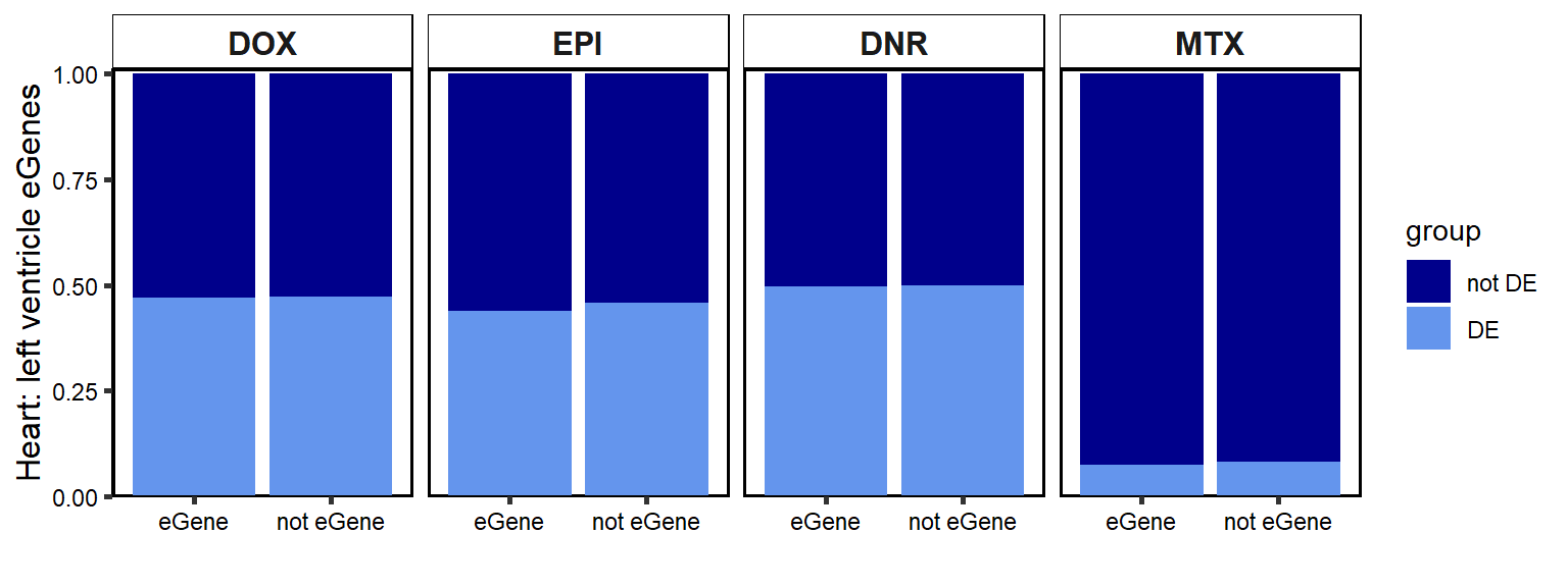
Additonal GTEx analysis and code is found here
B. 24 hour DEG enrichment in DOX-iPSC-DM eGenes
knowles4 <-readRDS("output/knowles4.RDS")
knowles5 <-readRDS("output/knowles5.RDS")
Knowles_count <-
  toplistall %>%
  mutate(id = dplyr::case_match(id, "Daunorubicin"~"DNR",
                                "Doxorubicin"~"DOX",
                                "Epirubicin"~"EPI",
                                "Mitoxantrone"~"MTX",
                                "Trastuzumab"~"TRZ",
                                "Vehicle"~"VEH",
                                .default = id)) %>%
  filter(id!='TRZ') %>%
  mutate(id=factor(id, levels = c('DOX','EPI','DNR','MTX','TRZ','VEH'))) %>%
  mutate(time=factor(time, levels=c("3_hours","24_hours"))) %>%
  group_by(time, id) %>%
  mutate(K4 = if_else(ENTREZID %in% knowles4$entrezgene_id,1,0))%>%
  mutate(K5 = if_else(ENTREZID %in% knowles5$entrezgene_id,1,0))%>%
  filter(adj.P.Val<0.05) %>%
  dplyr::summarize(n=n(), K4=sum(K4), K5=sum(K5)) %>%
  as.tibble() %>%
  dplyr::select(time,id,K4,K5) %>%
  rename("K4_y"='K4',"K5_y"='K5') %>%
  mutate(time = case_match(time, '3_hours'~'3 hrs',
                           '24_hours'~'24 hrs',
                           .default = time)) %>%
  mutate(K4_n= 417-K4_y, K5_n=273-K5_y) %>%
  pivot_longer(!c(time,id),
               names_to='QTL',
               values_to="gene_count") %>%
  separate(QTL,into=c("QTL_type",'group'),sep = '_') %>%
  mutate(QTL_type =case_match(QTL_type,
                              'K4'~'base\neGenes',
                              'K5'~'response\neGenes',.default = QTL_type)) %>%
  mutate(time=factor(time, levels=c("3 hrs","24 hrs"))) %>%
  group_by(id,time,QTL_type) %>%
  mutate(percent=gene_count/sum(gene_count)*100)  %>%
  ungroup() %>%
  filter(time=="24 hrs") %>%
  mutate(id=factor(id, levels = c('DOX','EPI','DNR','MTX','TRZ','VEH'))) %>%  mutate(group=factor(group, levels= c("n","y"), labels=c("not DE","DE")))


  ggplot(Knowles_count, aes(x=QTL_type,y=gene_count, group=group,  fill=group))+
    geom_col(position='fill')+
    facet_wrap(~id,nrow=1,ncol=4)+
    theme_classic()+
    ylab("iPSC-CM DOX eGenes ")+
    xlab(" ")+
    scale_color_manual(values=drug_palspc)+
    scale_fill_manual(values=drug_palspc)+
    scale_y_continuous( expand = expansion(c(0, 0.01))) +
    theme(strip.background = element_rect(fill = "white",
                                        linetype=1,
                                        linewidth = 0.5),
        plot.title = element_text(size=12,
                                  hjust = 0.5,
                                  face="bold"),
        axis.title = element_text(size = 12,
                                  color = "black"),
        axis.ticks = element_line(linewidth = 1.0),
        axis.text = element_text(color = "black"),
        panel.background = element_rect(colour = "black",
                                        size=1),
        strip.text.x = element_text(size=12,
                                    face = "bold"))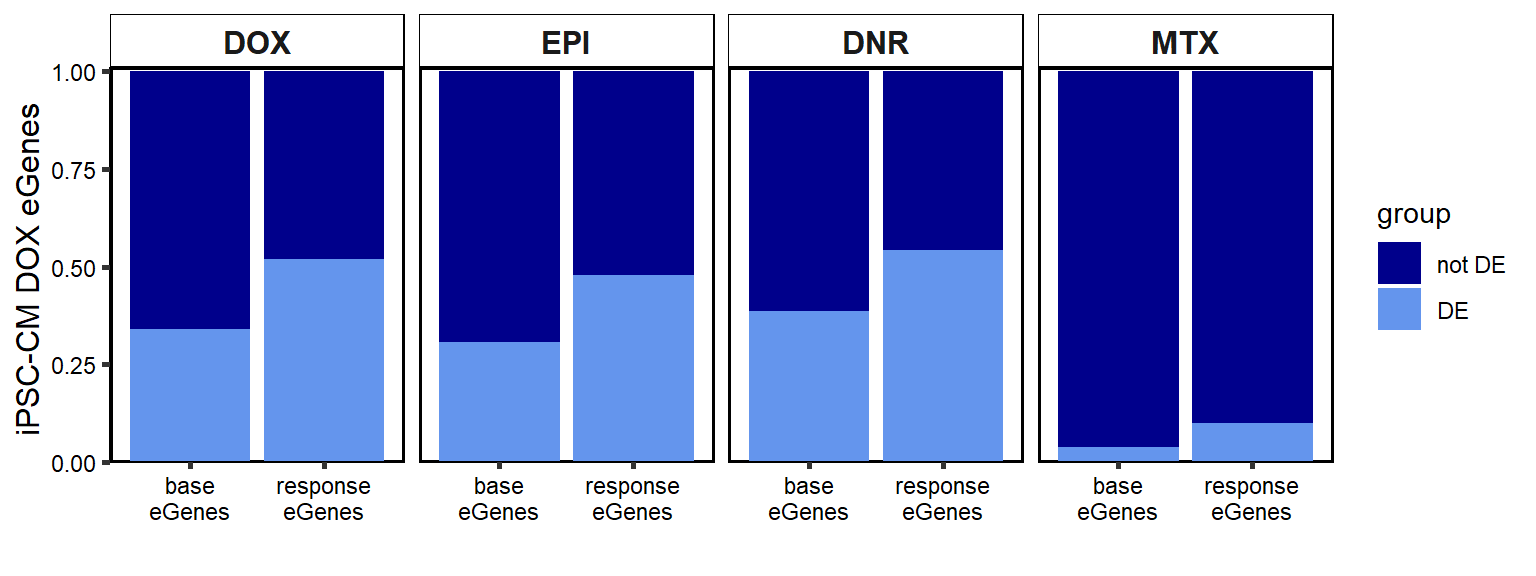
Additonal analysis and code for the Knowles data is found here
C. DOXreQTLS strongly overlap other TOP2i drugs
DOXreQTLs <- readRDS("output/DOXreQTLs.RDS")

assignInNamespace(x="plot_venn", value=plot_venn, ns="ggVennDiagram")

reQTL_overlapDE24 <- list(DOXreQTLs$ENTREZID,sigVDA24$ENTREZID, sigVEP24$ENTREZID, sigVMT24$ENTREZID)
re_incommon <- c(DOXreQTLs$ENTREZID,sigVDA24$ENTREZID, sigVEP24$ENTREZID, sigVMT24$ENTREZID)

names(reQTL_overlapDE24) <- c("Dox_reQTLS", "DNR DEGs","EPI DEGs","MTX DEGs")

DEG_incommon <-c(sigVDA24$ENTREZID, sigVEP24$ENTREZID, sigVMT24$ENTREZID)
uniqueDEGs_incommon <- unique(DEG_incommon)
two_venn <- list( DOXreQTLs$ENTREZID,uniqueDEGs_incommon)

ggVennDiagram::ggVennDiagram(two_venn,
                             category.names = c("DOX egenes\nn = 142","union of TOP2i DEGs\n     n = 7838"),
              show_intersect = FALSE,
              set_color = "black",
              category_size = c(6,6),
              label = "count",
              label_percent_digit = 1,
              label_size = 4,
              label_alpha = 0,
              label_color = "black",
              edge_lty = "solid", set_size = 4.5)+
  scale_x_continuous(expand = expansion(mult = .3))+
  scale_y_continuous(expand = expansion(mult = .1))+
   scale_fill_distiller(palette="Spectral", direction = -1, limits= c(1,200),oob=scales::squish)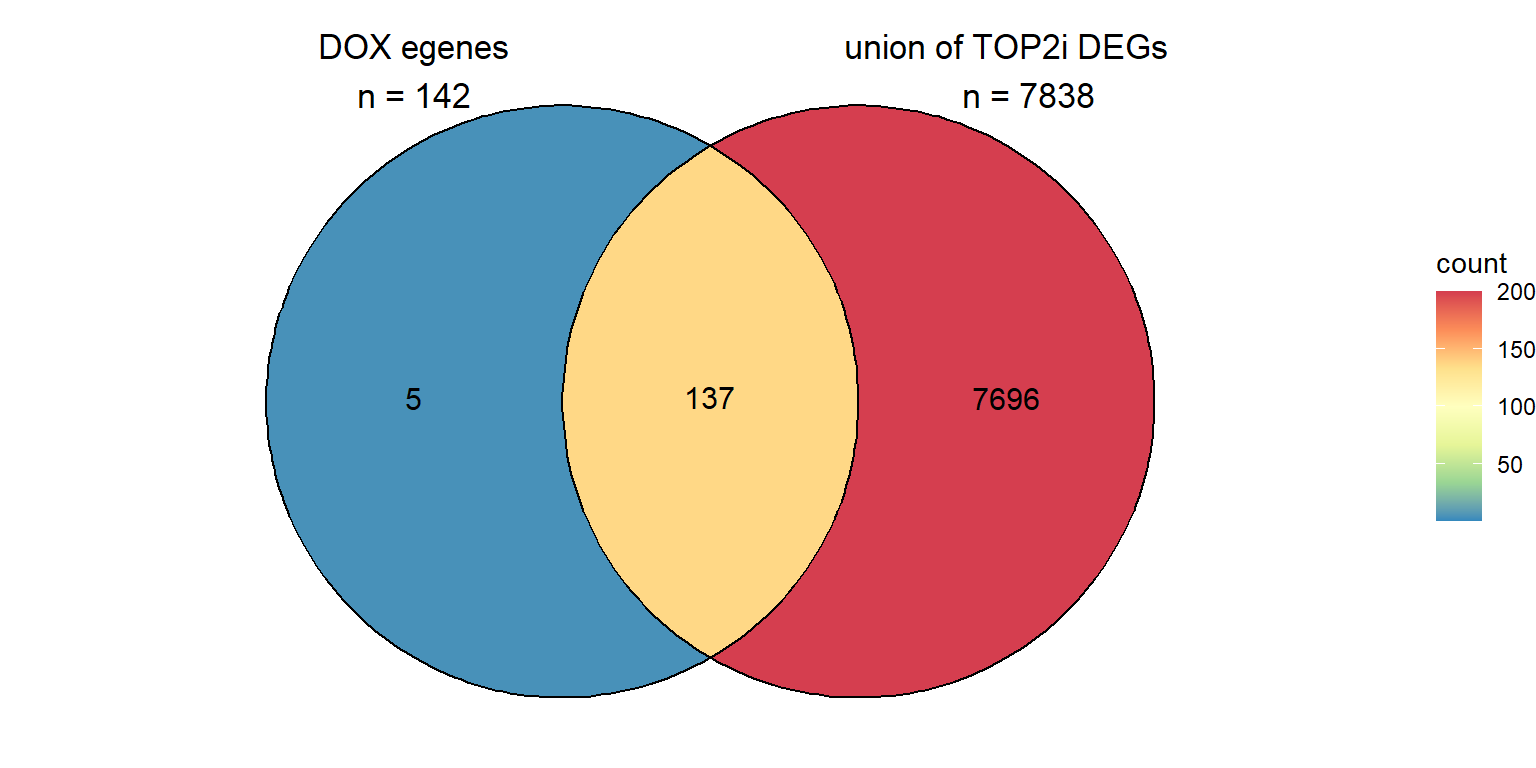
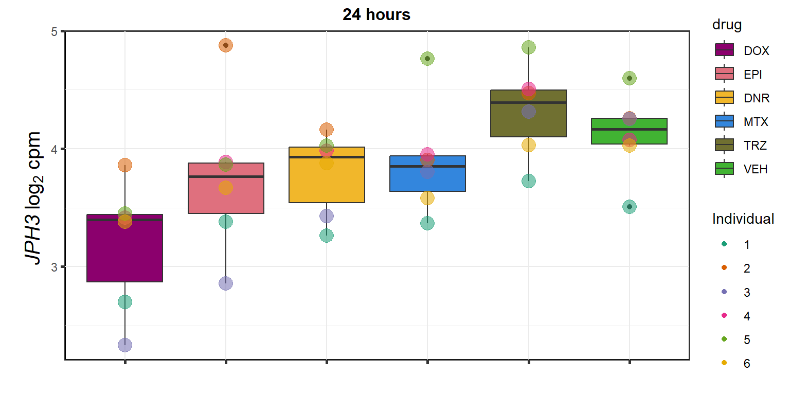
D. Stringently idetified DOX-only DE genes and DOX egenes only share JPH3
cpm_boxplot24h <-
  function(cpmcounts,
           GOI,
           brewer_palette,
           fill_colors,
           ylab) {
    ##GOI needs to be ENTREZID
    df <- cpmcounts
    df_plot <- df %>%
      dplyr::filter(rownames(.) == GOI) %>%
      pivot_longer(everything(),
                   names_to = "treatment",
                   values_to = "counts") %>%
      separate(treatment, c("drug", "indv", "time")) %>%
      mutate(time = case_match(time, "24h" ~ "24 hours", "3h" ~ "3 hours")) %>%
      mutate(indv = factor(indv, levels = c(1, 2, 3, 4, 5, 6))) %>%
      mutate(
        drug = case_match(
          drug,
          "Da" ~ "DNR",
          "Do" ~ "DOX",
          "Ep" ~ "EPI",
          "Mi" ~ "MTX",
          "Tr" ~ "TRZ",
          "Ve" ~ "VEH",
          .default = drug
        )
      ) %>%
      mutate(drug = factor(drug, levels = c('DOX', 'EPI', 'DNR', 'MTX', 'TRZ', 'VEH'))) %>%
      dplyr::filter(time == "24 hours")
    plot <- ggplot2::ggplot(df_plot, aes(x = drug, y = counts)) +
      geom_boxplot(position = "identity", aes(fill = drug)) +
      geom_point(aes(
        col = indv,
        size = 2,
        alpha = 0.5
      )) +
      guides(alpha = "none", size = "none") +
      scale_color_brewer(palette = brewer_palette, name = "Individual") +
      scale_fill_manual(values = fill_colors) +
      # facet_wrap("time", nrow=1, ncol=2)+
      theme_bw() +
      ylab(ylab) +
      xlab("") +
      ggtitle("24 hours") +
      theme(
        strip.background = element_rect(
          fill = "white",
          linetype = 1,
          linewidth = 0.5
        ),
        plot.title = element_text(
          size = 12,
          hjust = 0.5,
          face = "bold"
        ),
        axis.title = element_text(
          size = 15,
          color = "black",
          face = "bold"
        ),
        axis.ticks = element_line(linewidth = 1.0),
        panel.background = element_rect(colour = "black", size = 1),
        axis.text.x = element_blank(),
        strip.text.x = element_text(margin = margin(2, 0, 2, 0, "pt"), face = "bold")
      )
    print(plot)
  }
cpm_boxplot24h(cpmcounts,
               GOI = '57338',
               "Dark2",
               drug_pal_fact,
               ylab = (expression(atop(
                 " ", italic("JPH3") ~ log[2] ~ "cpm "
               ))))
For additional stringently identified genes, you can visit the supplementary data here or analysis located here.
sessionInfo()R version 4.3.1 (2023-06-16 ucrt)
Platform: x86_64-w64-mingw32/x64 (64-bit)
Running under: Windows 10 x64 (build 19045)
Matrix products: default
locale:
[1] LC_COLLATE=English_United States.utf8
[2] LC_CTYPE=English_United States.utf8
[3] LC_MONETARY=English_United States.utf8
[4] LC_NUMERIC=C
[5] LC_TIME=English_United States.utf8
time zone: America/Chicago
tzcode source: internal
attached base packages:
[1] stats graphics grDevices utils datasets methods base
other attached packages:
[1] paletteer_1.5.0 ggVennDiagram_1.2.3 broom_1.0.5
[4] RColorBrewer_1.1-3 ggsignif_0.6.4 cowplot_1.1.1
[7] data.table_1.14.8 BiocGenerics_0.46.0 lubridate_1.9.2
[10] forcats_1.0.0 stringr_1.5.0 dplyr_1.1.3
[13] purrr_1.0.2 readr_2.1.4 tidyr_1.3.0
[16] tibble_3.2.1 ggplot2_3.4.3 tidyverse_2.0.0
[19] workflowr_1.7.1
loaded via a namespace (and not attached):
[1] gtable_0.3.4 xfun_0.40 bslib_0.5.1 processx_3.8.2
[5] callr_3.7.3 tzdb_0.4.0 vctrs_0.6.3 tools_4.3.1
[9] ps_1.7.5 generics_0.1.3 proxy_0.4-27 fansi_1.0.4
[13] pkgconfig_2.0.3 KernSmooth_2.23-22 lifecycle_1.0.3 farver_2.1.1
[17] compiler_4.3.1 git2r_0.32.0 munsell_0.5.0 getPass_0.2-2
[21] httpuv_1.6.11 class_7.3-22 htmltools_0.5.6 sass_0.4.7
[25] yaml_2.3.7 later_1.3.1 pillar_1.9.0 jquerylib_0.1.4
[29] whisker_0.4.1 classInt_0.4-10 cachem_1.0.8 tidyselect_1.2.0
[33] digest_0.6.33 stringi_1.7.12 sf_1.0-14 rematch2_2.1.2
[37] labeling_0.4.3 rprojroot_2.0.3 fastmap_1.1.1 grid_4.3.1
[41] colorspace_2.1-0 cli_3.6.1 magrittr_2.0.3 utf8_1.2.3
[45] e1071_1.7-13 withr_2.5.0 RVenn_1.1.0 scales_1.2.1
[49] promises_1.2.1 backports_1.4.1 timechange_0.2.0 rmarkdown_2.24
[53] httr_1.4.7 hms_1.1.3 evaluate_0.21 knitr_1.44
[57] rlang_1.1.1 Rcpp_1.0.11 DBI_1.1.3 glue_1.6.2
[61] rstudioapi_0.15.0 jsonlite_1.8.7 R6_2.5.1 units_0.8-4
[65] fs_1.6.3